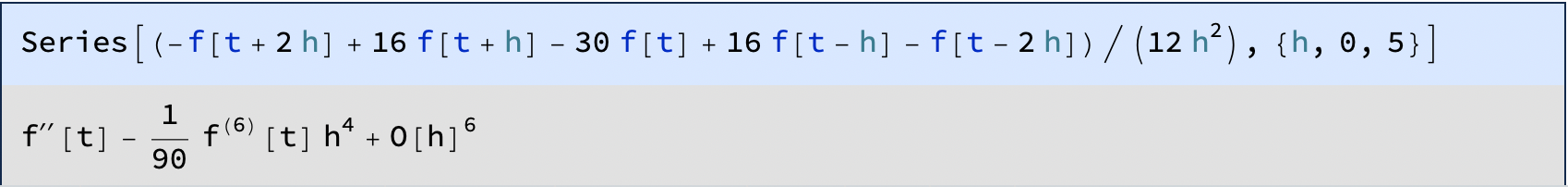
Use Taylor series expansions to verify the approximations
| (1) |
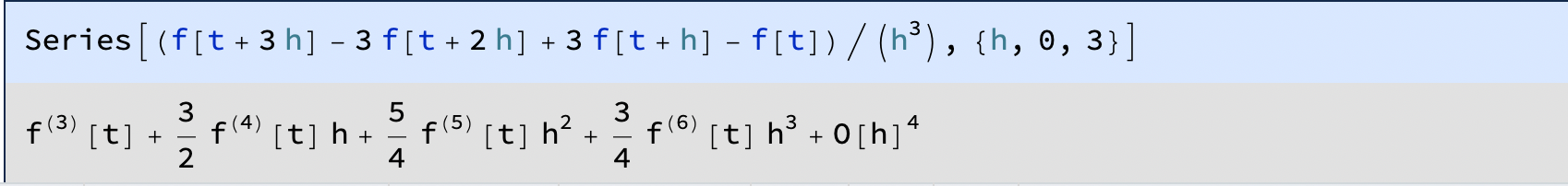
| (2) |
Determine the error term. Construct the polynomial approximant whose derivative leads to the above formula. Conduct a convergence study as for at , and compare the observed order of convergence with the theoretical estimate.
Solution. For hand computation, organize Taylor series expansions into a table with the coefficients from the finite difference formula. Observe that Taylor series terms of even powers in cancel out, and those of odd powers from simply double those from parts of the expansions. The power of multiplying is . Observing and exploiting such symmetries reduces the number of calculations considerably.
Deduce leading-order error
This can be verified in Mathematica.

Set origin at . Formula (1) contains data with . for a total of 5 conditions that can be satisfied by polynomial of degree .
This exercise highlights use of the Lagrange form of a Hermite interpolating polynomial with differing types of information at each node. The Lagrange basis functions
satisfy the desired conditions leading to the polynomial
A similar analysis can be applied to the second formula giving the error term
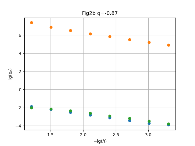
Steps for the convergence study:
Define the finite difference derivative approximations
Define the specified study functions
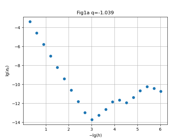
Define a function to construct the convergence plot by: evaluating the error
for , , extracting the order of convergence by least squares (linear regression)
and plotting the observed behavior.
∴ |
function conv(h0,t,f,D,N,fname,figname)
  df=zeros(N+1,1); u=zeros(N,1); h=h0; lgh=zeros(N+1,1)
  for k=1:N+1
    h=h/2; lgh[k]=log10(h); df[k]=D(t,f,h);
  end
  A=ones(N,2); x=-lgh[1:N]; A[:,2]=x;
  u[1:N]=log10.(abs.(df[2:N+1]-df[1:N]));
  q = floor((A\u)[2]*1000)/1000;
  plot(x,u,"o"); grid("on"); title(figname*" q="*string(q))
  xlabel(L"$-\lg(h)$"); ylabel(L"\lg(e_k)")
  savefig(fname)
  return q
end; |
∴ |

∴ |
figdir=homedir()*"/courses/MATH661/homework/H08/"; |
∴ |
clf(); h0=1; t0=1; conv(h0,t0,f1,D1,20,figdir*"H08Fig1a.png","Fig1a"); |
∴ |
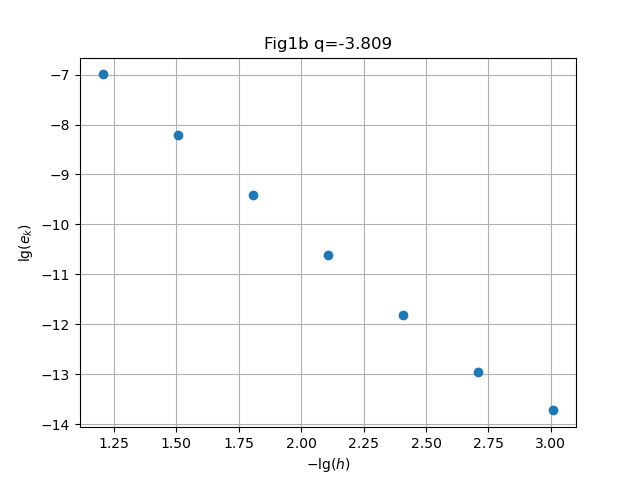
clf(); h0=1/8; conv(h0,t0,f1,D1,7,figdir*"H08Fig1b.png","Fig1b"); |
∴ |
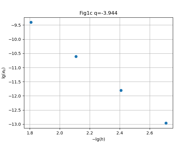
clf(); h0=1/32; conv(h0,t0,f1,D1,4,figdir*"H08Fig1c.png","Fig1c"); |
∴ |
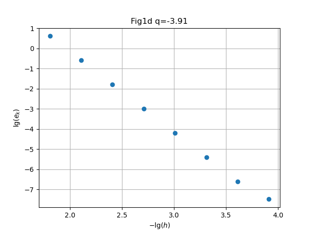
clf(); h0=1/32; conv(h0,t0,f2,D1,8,figdir*"H08Fig1d.png","Fig1d"); |
∴ |
clf(); h0=1/32; conv(h0,t0,f3,D1,8,figdir*"H08Fig1e.png","Fig1e"); |
∴ |
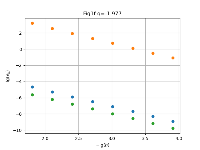
clf(); h0=1/32; conv(h0,t0,f1,D2,8,figdir*"H08Fig1f.png","Fig1f"); |
∴ |
h0=1/32; conv(h0,t0,f2,D2,8,figdir*"H08Fig1f.png","Fig1f"); |
∴ |
h0=1/32; conv(h0,t0,f3,D2,8,figdir*"H08Fig1f.png","Fig1f"); |
∴ |
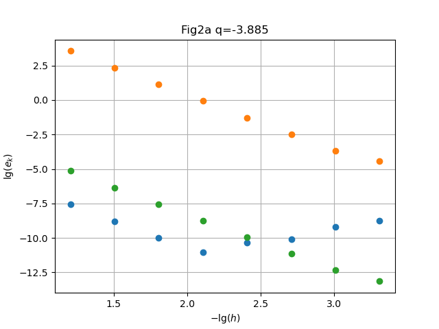
As above for
Solution. Symbolic computation in Mathematica readily gives , behavior respectively.
Define the finite difference derivative approximations
Construct a recursive function RecInt(a,b,err,f,Q) that has arguments scalars and functions and approximates
through repeated application of quadrature rule according to the algorithm
Algorithm
Recursive quadrature
RecInt(a,b,err,f,Q)
if
return
else
return RecInt(a,c,err,f,Q)+RecInt(c,b,err,f,Q)
Test the recursive integration procedure with trapezoid, Simpson, and Gauss-Legendre rules of orders 2,3 on the integral
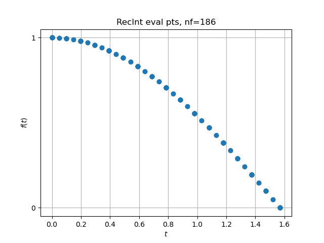
For each case, present plots of the integrand and the evaluation points used in the recursive quadrature algorithm. Construct convergence plots by executing the algorithm for various error thresholds and recording the number of evaluation points . Plot and comment on whether the observed order of convergence is that predicted by theoretical quadrature error estimates.
Solution. Define:
Recursive quadrature procedure
∴ |
function RecInt(a,b,eps,f,Q,level)
  global nf,nmax,lmax
  c=a+(b-a)/2; Qab=Q(a,b,f); Qac=Q(a,c,f); Qcb=Q(c,b,f)
  new=Qac+Qcb; old=Qab;
  if nf > nmax/2 return new end
  if level > lmax return new end
  err=abs((new-old)/new)
  if err<eps
    return new
  else
    return RecInt(a,c,eps,f,Q,level+1)+RecInt(c,b,eps,f,Q,level+1)
  end
end; |
∴ |
Quadrature rules:
Trapezoid
∴ |
function trapezoid(a,b,f) return 0.5*(b-a)*(f(a)+f(b)) end; |
∴ |
Simpson
∴ |
function simpson(a,b,f) return (b-a)/6 * (f(a)+4*f(0.5*(a+b))+f(b)) end; |
∴ |
Gauss-Legendre 2
∴ |
function gl2(a,b,f) s=(b-a)/2; z(t)=s*(t+1)+a; s3=sqrt(1/3); return s*(f(z(-s3))+f(z(s3))) end; |
∴ |
Gauss-Legendre 3
∴ |
function gl3(a,b,f) s=(b-a)/2; z(t)=s*(t+1)+a; s35=sqrt(3/5); w1=5/9; w0=8/9 return s*(w1*f(z(-s35)) + w0*f(z(0)) + w1*f(z(s35))) end; |
∴ |
Define the integrand. Each time the integrand is called record the evaluation point and increment a counter of function evaluations. The integrand is singular at , but over an interval of measure zero in the limit. Hence setting the integrand value to zero at does not affect the integral value. Also define a simpler integrand for overall testing.
∴ |
function f(t)
  global nf,tvals,fvals
  if abs(t)<1.0e-6
    fval=0.
  else
    fval=cos(1/t)
  end
  nf = nf+1; tvals[nf]=t; fvals[nf]=fval
  return fval
end; |
∴ |
function g(t) global nf,tvals,fvals fval = cos(t) nf = nf+1; tvals[nf]=t; fvals[nf]=fval return fval end; |
∴ |
Initialize function evaluation counter, values, call the routine for simple integrand
Initialize function evaluation counter, values, call the routine for singular integrand
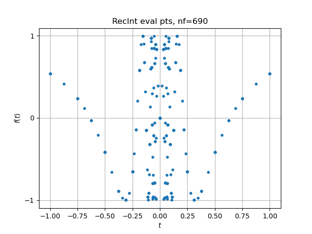 |
Figure 4. For integrand function evaluation points are clustered in regions of rapid variation of the function. Within a limit on the number of function evaluation , only the GL3 quadrature gives a value of -0.16 with two accurate digits. This example highlights both recursive quadrature and the need for specialized numerical quadrature procedures for highly oscillatory or singular integrands. |
∴ |
global nf,nmax,lmax |
∴ |
nf=0; nmax=100000; lmax=8; tvals=zeros(nmax,1); fvals=zeros(nmax,1); |
∴ |
Qg=RecInt(-1,1,10.0^(-1),f,trapezoid,0); [nf Qg] |
(7)
∴ |
clf(); plot(tvals[1:nf],fvals[1:nf],"."); |
∴ |
xlabel(L"$t$"); ylabel(L"$f(t)$"); grid("on"); |
∴ |
title("RecInt eval pts, nf="*string(nf)); |
∴ |
figdir=homedir()*"/courses/MATH661/homework/H08/"; |
∴ |
savefig(figdir*"Fig3fT.png"); |
∴ |
nf=0; nmax=1000000; lmax=32; tvals=zeros(nmax,1); fvals=zeros(nmax,1); |
∴ |
Qg=RecInt(-1,1,10.0^(-2),f,trapezoid,0); [nf Qg] |
(8)
∴ |
nf=0; nmax=1000000; lmax=32; tvals=zeros(nmax,1); fvals=zeros(nmax,1); |
∴ |
Qg=RecInt(-1,1,10.0^(-2),f,simpson,0); [nf Qg] |
(9)
∴ |
nf=0; nmax=1000000; lmax=32; tvals=zeros(nmax,1); fvals=zeros(nmax,1); |
∴ |
Qg=RecInt(-1,1,10.0^(-2),f,gl2,0); [nf Qg] |
(10)
∴ |
nf=0; nmax=1000000; lmax=32; tvals=zeros(nmax,1); fvals=zeros(nmax,1); |
∴ |
Qg=RecInt(-1,1,10.0^(-2),f,gl3,0); [nf Qg] |
(11)
∴ |
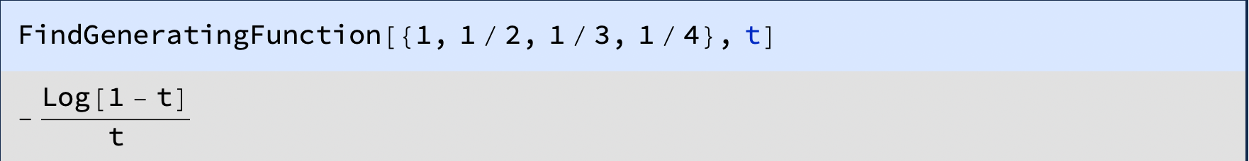 The generating
function has been found using only 4 terms. Extra credit (4 pts).
Can you find generating functions for ?
The generating
function has been found using only 4 terms. Extra credit (4 pts).
Can you find generating functions for ?