Investigate various aspects of the $Ly=f\left(y\right)$ problem with $L$ a linear operator and $f$ nonlinear. Algorithms will be applied to the Van der Pol oscillator for $t\in [0,250]$ with $\mu =1$,

Plots of the solution are typically presented in phase space as (x(t),x'(t)).

1Track 1

1. Rewrite the second-order ODE as a system of first-order equations ${𝒚}^{\text{'}}=𝒇(t,𝒚)$.

   Solution. Denote $x^{\text{'}}=w$, and obtain system

   ${\displaystyle \{\begin{array}{lll}{x}^{\text{'}}& =& w\\ w^{\text{'}}& =& -x+\mu (1-x^2)w\end{array}.,{𝒚}^{\text{'}}=\frac{d}{dt}\left[\begin{array}{l}x\\ w\end{array}\right]=\left[\begin{array}{l}w\\ -x+\mu (1-x^2)w\end{array}\right]=𝒇\left(𝒚\right),𝒚=\left[\begin{array}{l}x\\ w\end{array}\right],{𝒚}_0=\left[\begin{array}{l}0\\ 1\end{array}\right].}$

   Note that the slope function $𝒇$ does not explicitly depend on $t$, the system is said to be autonomous.

2. Carry out a convergence study when applying the single-step Runge-Kutta method

   ${\displaystyle {𝒚}_{n+1}={𝒚}_n+\frac{1}{6}({𝒌}_1+2{𝒌}_2+2{𝒌}_3+{𝒌}_4),}$ ${\displaystyle \begin{array}{c}{𝒌}_1=h𝒇(t_n,{𝒚}_n)\\ {𝒌}_2=h𝒇(t_n+\frac{1}{2}h,{𝒚}_n+\frac{1}{2}{𝒌}_1)\\ {𝒌}_3=h𝒇(t_n+\frac{1}{2}h,{𝒚}_n+\frac{1}{2}{𝒌}_2)\\ {𝒌}_4=h𝒇(t_n+h,{𝒚}_n+{𝒌}_3)\end{array}}$

   Solution.

   Notes:

   • Convergence of a numerical ODE solution requires consistency and stability. Linear stability, i.e., stability for the linearized ODE is required for stability. Whenever carrying out an ODE numerical solution a preliminary stability analysis is required to determine step sizes required for stability and accuracy.

   • The Julia implementation closely follows the above mathematical formulation. Sub-tasks within the problem are encapsulated into Julia functions. Each task is implemented and subsequently tested. Julia variables closely follow the mathematical notation.

   Linearization of $𝒇$ leads to

   ${\displaystyle {𝒚}^{\text{'}}=𝒇\left(𝒚\right)\cong 𝒇\left({𝒚}_0\right)+𝑱\left({𝒚}_0\right)(𝒚-{𝒚}_0)}$

   where $𝑱\left(𝒚\right)$ is the Jacobian

   ${\displaystyle 𝑱\left(𝒚\right)=\frac{\partial 𝒇}{\partial 𝒚}\left(𝒚\right)=\left[\begin{array}{ll}0& 1\\ -1-2\mu xw& \mu (1-x^2)\end{array}\right].}$

   The standard harmonic oscillator $x^{\text{'}\text{'}}+x=0$ is obtained for $\mu =0$, and is useful for testing numerical algorithms and gaining insight into the nonlinear Von der Pol oscillator.

   Convergence requires that $z=\lambda h$ lie within the domain of stability of a particular scheme. The eigenvalues of $𝑱\left(𝒚\right)$ are roots of

   ${\displaystyle \left|\begin{array}{ll}\lambda & -1\\ 1+2\mu xw& \lambda -\mu (1-x^2)\end{array}\right|={\lambda }^2-\mu (1-x^2)\lambda +1+2\mu xw=0.}$

   An immediate observation is that for $\mu =0$, $𝑱$ is skew-symmetric and hence has purely imaginary eigenvalues, namely ${\lambda }_{1,2}=\pm i$, roots of

   ${\displaystyle {\lambda }^2+1=0.}$

   $•$Define linearized problem eigenvalues

   ∴	function λ(μ,x,w) a=1; b=-μ*(1-x^2); c=1+2*μ*x*w Δ = Complex(b^2-4*a*c) return [-b-sqrt(Δ) -b+sqrt(Δ)]/2 end;

   ∴

   λ(0,0,1)

   ${\displaystyle \left[\begin{array}{cc}-\text{i}& \text{i}\end{array}\right]}$

   (1)

   ∴

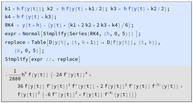
   Fourth-order Runge-Kutta applied to the model problem $f\left(y\right)=\lambda y$ gives

   ${\displaystyle \begin{array}{c}{k}_1=z{y}_n=p_1\left(z\right)y_n\\ k_2=z(y_n+\frac{1}{2}z{y}_n)=z(1+\frac{z}{2})y_n=p_2\left(z\right)y_n=z(1+\frac{1}{2}{p}_1\left(z\right))y_n\\ k_3=z(y_n+\frac{1}{2}z(1+\frac{z}{2})y_n)=z(1+\frac{1}{2}z(1+\frac{z}{2}))y_n=p_3\left(z\right)y_n=z(1+\frac{1}{2}{p}_2\left(z\right))y_n\\ k_4=z(1+z(1+\frac{1}{2}z(1+\frac{z}{2})))y_n=p_4\left(z\right)y_n=z(1+p_3\left(z\right))y_n\end{array}}$

   ${\displaystyle y_{n+1}=[1+\frac{1}{6}(p_1\left(z\right)+2p_2\left(z\right)+2p_3\left(z\right)+p_4\left(z\right))]y_n=P\left(z\right)y_n.}$

   ${\displaystyle P\left(z\right)=1+z+\frac{1}{2}{z}^2+\frac{1}{6}{z}^3+\frac{1}{24}{z}^4}$

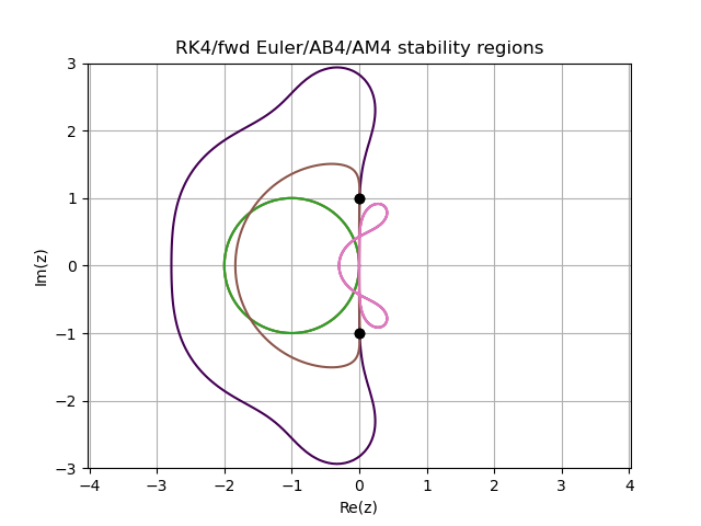
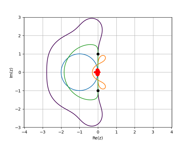
   Stability requires $\left|P\left(z\right)\right|⩽1$. The stability boundary locus is obtained when $\left|P\left(z\right)\right|=1$, and can be ascertained from a contour plot of $\left|P\left(z\right)\right|$ (Fig. 1).

   $•$

   Figure 1. Stability boundary for Runge-Kutta (outer), Adams-Bashforth (inner), Adams-Moulton (middle) of fourth order and forward Euler (circle). The points $z_{1,2}=\pm i$ are also represented that correspond to the harmonic oscillator roots ${\lambda }_{1,2}$ and step size $h=1$. Interpret this to state that forward Euler and AB4 would be unstable at step size $h=1$, while AM4 and RK4 would be stable. Further note that forward Euler is always unstable for the harmonic oscillator

   ∴

   function BLplot(nfig) np=100; x=range(-3,3,np); y=range(-3,3,np); absP=zeros(np,np); P(z)=1+z+z^2/2+z^3/6+z^4/24; for i=1:np for j=1:np local z z=x[i]+Complex(0,1)*y[j] absP[i,j]=abs(P(z)) end end xgrid=repeat(x',np,1) ygrid=repeat(y,1,np) figure(nfig); clf(); contour(xgrid,ygrid,absP',[1.0]) grid("on"); axis("equal"); xlabel("Re(z)"); ylabel("Im(z)") θ=0:0.01:2*pi; x=-1 .+ cos.(θ); y=sin.(θ); plot(x,y) ρAB4(z)=z^4-z^3; σAB4(z)=(55*z^3-59*z^2+37*z-9)/24 ρAM4(z)=z^4-z^3; σAM4(z)=(251*z^4+646*z^3-264*z^2+106*z-19)/720 ζ=exp.(Complex(0,1)*θ) zBLAB4=ρAB4.(ζ) ./ σAB4.(ζ) plot(real.(zBLAB4),imag.(zBLAB4)) zBLAM4=ρAM4.(ζ) ./ σAM4.(ζ) plot(real.(zBLAM4),imag.(zBLAM4)) plot([0 0],[-1 1],"ko") title("RK4/fwd Euler/AB4/AM4 stability regions") end;

   ∴	figdir=homedir()*"/courses/MATH661/homework/H09/";

   ∴	BLplot(2);

   ∴	savefig(figdir*"schemesBL.png");

   $•$

   Figure 2. Eigenvalues $\lambda$ of the linearized Van der Pol oscillator for $x,w\in [-2.5,2.5]$ represented as $z=h\lambda$ for $h=0.2$. Smaller step sizes will maintain the shape of the eigenvalue point cloud, but reduce its size. Instability is possible but whether it is actually observed during time integration depends on the actual $x,x^{\text{'}}$ values on a specific trajectory.

   ∴	np=50; x=range(-2.5,2.5,np); w=range(-2.5,2.5,np);

   ∴	reλVdP=zeros(np,np,2); imλVdP=zeros(np,np,2); h=0.2;

   ∴	for i=1:np for j=1:np λij=h*λ(1,x[i],w[j]) reλVdP[i,j,1:2]=real.(λij) imλVdP[i,j,1:2]=imag.(λij) end end

   ∴	reλpts=reshape(reλVdP,2*np*np,1); imλpts=reshape(imλVdP,2*np*np,1);

   ∴	plot(reλpts,imλpts,"r.");

   ∴	savefig(figdir*"VdPBL.png");

   $•$Define problem initial condition

   ∴	μ=1; t0=0; t1=250; y0=zeros(2,1); y0[2,1]=1; y0

   ${\displaystyle \left[\begin{array}{c}0.0\\ 1.0\end{array}\right]}$

   (2)

   ∴	nNSmax=2^20; λNS=Array{Complex}(undef,nNSmax,1); nNS=0;

   ∴

   $•$Define the function $𝒇$ for the Van der Pol and harmonic oscillators. Maintain a record of the linearized Van der Pol eigenvalues

   ∴	function fVdPcnt(t,y) global μ,λNS,nNS f=zeros(2,1); x=y[1]; w=y[2]; f[:,1]=[w; -x+μ*(1-x*x)*w] λ12=λ(μ,x,w) nNS=nNS+1; λNS[nNS]=λ12[1] nNS=nNS+1; λNS[nNS]=λ12[2] return f end;

   ∴	function fVdP(t,y) global μ,λNS,nNS f=zeros(2,1); x=y[1]; w=y[2]; f[:,1]=[w; -x+μ*(1-x*x)*w] return f end;

   ∴	f0=fVdP(t0,y0)

   ${\displaystyle \left[\begin{array}{c}1.0\\ 1.0\end{array}\right]}$

   (3)

   ∴	function fH(t,y) f=zeros(2,1); x=y[1]; w=y[2]; f[:,1]=[w; -x] return f end;

   ∴

   fH(t0,y0)

   ${\displaystyle \left[\begin{array}{c}1.0\\ -0.0\end{array}\right]}$

   (4)

   ∴

   $•$Define the Runge-Kutta method

   ∴	function rk4(t,y,f,h,s=1) k1=h*f(t,y) k2=h*f(t+h/2,y+k1/2) k3=h*f(t+h/2,y+k2/2) k4=h*f(t+h,y+k3) return y+(k1+2*(k2+k3)+k4)/6 end;

   ∴	y1=rk4(t0,y0,fVdP,1)

   ${\displaystyle \left[\begin{array}{c}1.2415364583333333\\ 0.9983851114908854\end{array}\right]}$

   (5)

   ∴

   $•$Define a procedure to apply an $s$-step numerical scheme $L$ to construct an integral curve for $t\in [t_0,t_1]$. For Runge-Kutta $s=1$. For $s>1$ additional starting values are determined from using lower-order versions of the same scheme.

   ∴	function dsolve(t0,t1,nSteps,y0,f,L,s=1) h=(t1-t0)/nSteps; m=size(y0)[1] t=h*(0:nSteps) .+ t0; y=zeros(m,nSteps+1) y[1:m,1]=y0[1:m] for n=1:s-1 y[1:m,n+1]=L(t[n],y[1:m,n:-1:1],f,h,n) end for n=s:nSteps y[1:m,n+1]=L(t[n],y[1:m,n:-1:n-s+1],f,h,s) end return y end;

   ∴	dsolve(t0,t0+1,2,y0,fVdP,rk4)

   ${\displaystyle \left[\begin{array}{ccc}0.0& 0.6133200327555338& 1.2455899701904507\\ 1.0& 1.391127224106943& 0.9819591102115592\end{array}\right]}$

   (6)

   ∴

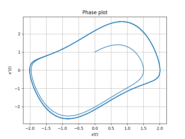
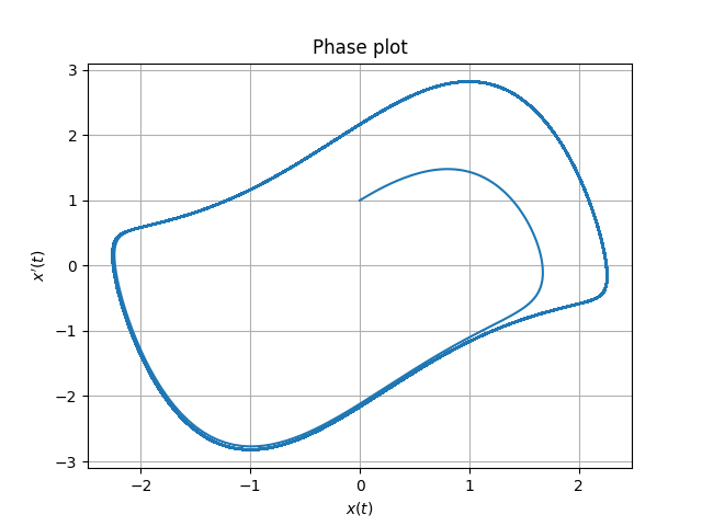
   $•$Define a procedure to plot the solution in phase space $(x\left(t\right),x^{\text{'}}\left(t\right))$

   Figure 3. Van der Pol oscillator phase plot

   Figure 4. Actually encountered $z=\lambda h$ values during RK4 solution.

   ∴	function pplot(y) plot(y[1,:],y[2,:]); grid("on"); xlabel(L"$x(t)$"); ylabel(L"$x'(t)$") title("Phase plot") end;

   ∴	clf(); nNS=0; pplot(dsolve(t0,t1,2^12,y0,fVdPcnt,rk4));

   ∴	figdir=homedir()*"/courses/MATH661/homework/H09/";

   ∴	savefig(figdir*"VdPsol1.png");

   ∴	clf(); pplot(dsolve(t0,t1,2^12,y0,fH,rk4)); axis("equal");

   ∴

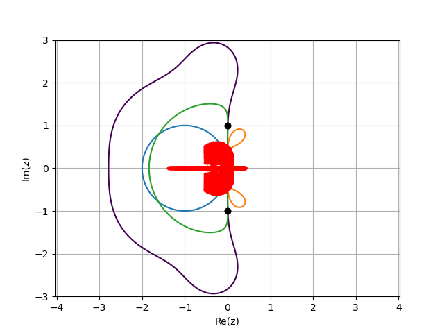
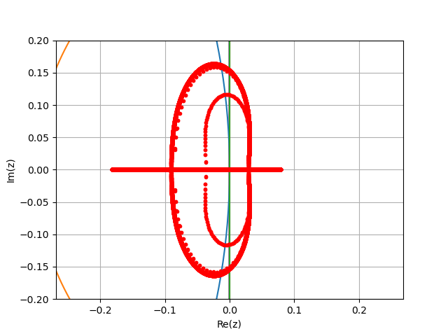
   Plot the actually encountered eigenvalues on the stability diagrams

   ∴	hNS=(t1-t0)/2^12;

   ∴	BLplot(2); plot(real.(hNS*λNS[1:nNS]),imag.(hNS*λNS[1:nNS]),"r.");

   ∴	savefig(figdir*"VdPRK4NS1.png");

   ∴	xlim(-0.2,0.2); ylim(-0.2,0.2);

   ∴	savefig(figdir*"VdPRK4NS2.png");

   ∴

   $•$Define a procedure to compute the error between two ODE solutions with steps sizes $h_2=h_1/2$. Division by the number of points makes this a one-step error.

   ∴	function dsolveErr(y1,y2) n1 = size(y1)[1] return norm(y2[1,1:2:2*n1]-y1[1,1:n1])/n1 end;

   ∴	y1=dsolve(t0,t1,2^11,y0,fVdP,rk4);

   ∴	y2=dsolve(t0,t1,2^12,y0,fVdP,rk4);

   ∴	y3=dsolve(t0,t1,2^13,y0,fVdP,rk4);

   ∴	[dsolveErr(y1,y2) dsolveErr(y2,y3)]

   ${\displaystyle \left[\begin{array}{cc}2.8892174840089435e-7& 8.66528815368639e-9\end{array}\right]}$

   (7)

   ∴

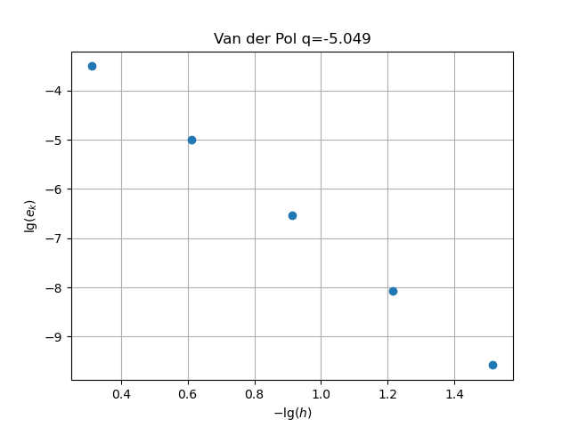
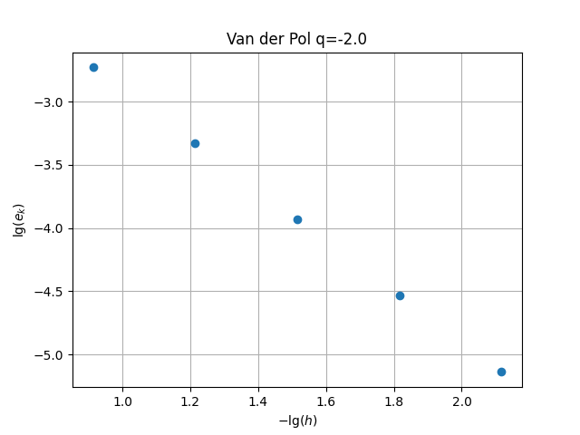
   $•$Define a procedure to construct a convergence plot by modification of the procedure from S08

   Figure 5. Convergence plot shows better than fifth-order one-step order, better than fourth-order global error for the Runge-Kutta scheme applied to the Van der Pol oscillator.

   ∴

   function conv(N0,N,fname,figname,L,s=1) global t0,t1 lgh=zeros(N,1); lgerr=zeros(N,1) for k=1:N nsteps=2^(N0+k) h=(t1-t0)/nsteps; lgh[k]=log10(h) y1=dsolve(t0,t1, nsteps,y0,fVdP,L,s) y2=dsolve(t0,t1,2*nsteps,y0,fVdP,L,s) lgerr[k]=log10(dsolveErr(y1,y2)) end A=ones(N,2); x=-lgh[1:N]; A[:,2]=x; q = floor((A\lgerr)[2]*1000)/1000; plot(x,lgerr,"o"); grid("on"); title(figname*" q="*string(q)) xlabel(L"$-\lg(h)$"); ylabel(L"\lg(e_k)") savefig(fname) return q end;

   ∴	figure(1); clf(); conv(10,5,figdir*"VdPconvRK4.png","Van der Pol",rk4)

   $-5.029$

   ∴

3. Carry out a convergence study when applying the Adams-Bashforth of order 4.

   Solution. Simply define a new numerical scheme and apply the procedures above. Runge-Kutta is a single-step method and produces a new $y_{n+1}$ from $y_n$,

   ${\displaystyle y_n\to y_{n+1}.}$

   Adams-Bashforth schemes of order $s$ are multistep, and can be considered to advance a vector with $s$ components

   ${\displaystyle \left[\begin{array}{llll}{y}_n& y_{n-1}& \dots & y_{n-(s-1)}\end{array}\right]\to \left[\begin{array}{llll}{y}_{n+1}& y_n& \dots & y_{n-s}\end{array}\right]}$

   $•$Define the Adams-Bashforth methods. The input argument $y$ is assumed to hold the most recent $s$ values

   Figure 6. (Left) Phase plot for AB4 solution with $2^{16}$ time steps. (Right) Convergence plot shows lower than theoretically predicted one-step error (explained by large number of eigenvalues outside stability region encountered during time advancement)

   ∴	bAB=[ 1 0 0 0; 3 -1 0 0; 23 -16 5 0; 55 -59 37 -9];

   ∴	w=diagm(0 => 1 ./ [1; 2; 12; 24]); bAB=w*bAB;

   ∴	function ab(t,y,f,h,s) global bAB ynew = y[:,1] for k=1:s ynew = ynew + h*bAB[k]*f(t,y[:,k]); t=t-h end return ynew end;

   ∴	clf(); nNS=0; pplot(dsolve(t0,t1,2^16,y0,fVdP,ab,4));

   ∴	savefig(figdir*"ab4sol.png")

   ∴	y1=dsolve(t0,t1,2^16,y0,fVdP,ab,4);

   ∴	y2=dsolve(t0,t1,2^17,y0,fVdP,ab,4);

   ∴	y3=dsolve(t0,t1,2^18,y0,fVdP,ab,4);

   ∴	[dsolveErr(y1,y2) dsolveErr(y2,y3)]

   ${\displaystyle \left[\begin{array}{cc}0.0014323304640129209& 0.000715710484655574\end{array}\right]}$

   (8)

   ∴	figure(1); clf(); conv(10,5,figdir*"VdPconvAB4.png","Van der Pol",ab)

   $-2.0$

   ∴

2Track 2

1. Rewrite the second-order ODE as a system of first-order equations ${𝒚}^{\text{'}}=𝒇(t,𝒚)$.

   Solution. See above.

2. Use a symbolic package (e.g., Mathematica) to verify the fourth-order theoretical accuracy of the Runge-Kutta method from Track 1.

   Solution. Try running the following instructions individually. Fifth order one-step error is obtained, implying fourth order glocal error.

   

3. Carry out a convergence study using Adams-Moulton of fourth order. This requires knowledge the latest value ${𝒚}_{n+1}$. Approximate this by a predictor ${\stackrel{\sim }{𝒚}}_{n+1}$ obtained by an Adams-Bashforth of fourth order where needed, e.g., $𝒇\left({𝒚}_{n+1}\right)\cong 𝒇\left({\stackrel{\sim }{𝒚}}_{n+1}\right)$.

   Solution. As above.