Scientific computation

Sorin Mitran

Department of Mathematics

University of North Carolina at Chapel Hill

Abstract

The goal of scientific computation is the construction of quantitatively verifiable models of the natural world. Scientific computation intertwines mathematics, algorithm formulation, software and hardware engineering with domain-specific knowledge from the physical, life, or social sciences. It is the fusion of these disciplines that imparts a distinct identity to scientific computing, and mathematical concepts must be complemented by practical modeling considerations to achieve successful computational simulation.

Human interpretation of the complexity of the natural world has historically led to parallel developments in formulation of abstract concepts, construction of models, and use of computational aids. This is the case on the long time span from prehistoric formulation of the abstract concept of a number and use of tally sticks, to current efforts based on quantum mechanics and superconducting qubit electronics. A dichtomy arises between the formulation of mathematical concepts asserted purely by reason and practicable predictions of the natural world. The conflicting approaches are reconciled by modeling and approximation. Domain sciences such as physics, biology, or sociology construct the relevant models. Comparison of model predictions to observation can sometimes be carried out through devices as simple as Galileo's inclined plane. The much higher complexity of models of airplane flight, or cancer progression, or activity on social media requires different tools, paradigmatically represented by the modern digital computer. In this more complex setting, scientific computing is instrumental in extracting verifiable predictions from models.

Central to computational prediction is the idea of approximation: finding a simple mathematical representation of some complex model of reality. Archimedes approximated the area of a parabolic segment by that an increasing number of inscribed triangles. Nowadays meteorological observations are input to a digital computer to predict future rainfall. The weather model implemented on the computer contains numerous approximations. Remarkably, both models rely on the same technique of additive approximation: summation of successive corrections to obtain increased accuracy.

One of the goals of this textbook is to highlight how computational methods arise as expressions of just a few approximation approaches. Additive corrections underlie many methods ranging from interpolation to numerical integration, and benefit from a remarkably complete theoretical framework within linear algebra. Alternatively, successive function composition is a distinct approximation idea, with a theoretical framework that is not yet complete, and whose expression leads to the burgeoning field of "machine learning". The process by which a specific approximation approach leads to different types of algorithms is a unifying theme of the presentation, and hopefully not only illuminates well-known algorithms, but also serves as a guide to future research.

The presentation of topics and ideas is at the graduate level of study, but with a focus on unifying ideas rather than detailed techniques. Much of traditional numerical methods and some associated analysis is presented and seen to be related to real analysis and linear algebra. The same theoretical framework can be extended to probability spaces and account for random phenomena. The nonlinear approach to approximation that characterizes artificial neural networks requires a different conceptual framework which has yet to be crystallized. Though numerical methods are prevalent in scientific computation, this text also considers alternatives that should be part of a computational scientist's toolkit such as symbolic, topological, and geometric computation.

Scientific computing is not a theoretical exercise, and successful simulation relies on acquiring the skill set to implement mathematical concepts and approximation techniques into efficient code. This text intersperses method presentation and implementation, mostly in the Julia language. An associated electronic version of his textbook uses the TeXmacs scientific editing platform to enable live documents with embedded computational examples, allowing immediate experimentation with the presented algorithms.

Abstract 5

I. Number Approximation 15

Lecture 1: Number Approximation 17

1.Numbers 17

1.1.Number sets 17

1.2.Quantification 17

1.3.Computer number sets 18

2.Approximation 21

2.1.Axiom of floating point arithmetic 21

2.2.Cummulative floating point operations 21

3.Successive approximations 23

3.1.Sequences in $ℝ$ 23

3.2.Cauchy sequences 25

3.3.Sequences in $𝔽$ 26

Summary. 26

Lecture 2: Approximation techniques 26

1.Rate and order of convergence 26

2.Convergence acceleration 30

2.1.Aitken acceleration 30

3.Approximation correction types 31

3.1.Additive corrections 32

3.2.Multiplicative corrections 32

3.3.Continued fractions 33

3.4.Composite corrections 33

Summary. 34

Lecture 3: Problems and Algorithms 34

1.Mathematical problems 34

1.1.Formalism for defining a mathematical problem 34

1.2.Vector space 36

1.3.Norm 36

1.4.Condition number 36

2.Solution algorithm 37

2.1.Accuracy 37

2.2.Stability 37

Summary. 38

II. Linear Approximation 39

1. Linear Algebra 43

Lecture 4: Linear Combinations 43

1.Finite-dimensional vector spaces 43

1.1.Overview 43

1.2.Real vector space $ℛ_{m}$ 43

Column vectors. 43

Row vectors. 44

Compatible vectors. 44

1.3.Working with vectors 44

Ranges. 44

2.Linear combinations 45

2.1.Linear combination as a matrix-vector product 45

Linear combination. 45

Matrix-vector product. 45

2.2.Linear algebra problem examples 45

Linear combinations in $E_{2}$ . 45

Linear combinations in $ℛ_{m}$ and $𝒞^{0} [0, 2 π)$ . 46

Summary. 47

Lecture 5: Linear Functionals and Mappings 48

1.Functions 48

1.1.Relations 48

Homogeneous relations. 48

1.2.Functions 48

1.3.Linear functionals 49

1.4.Linear mappings 50

2.Measurements 50

2.1.Equivalence classes 50

2.2.Norms 51

2.3.Inner product 53

3.Linear mapping composition 54

3.1.Matrix-matrix product 54

Lecture 6: Fundamental Theorem of Linear Algebra 56

1.Vector Subspaces 56

1.1.Definitions 56

1.2.Vector subspaces of a linear mapping 57

2.Linear dependence, vector space basis and dimension 59

2.1.Linear dependence 59

2.2.Basis and dimension 60

2.3.Dimension of matrix spaces 60

3.The FTLA 61

3.1.Partition of linear mapping domain and codomain 61

3.2.FTLA statement 62

Lecture 7: The Singular Value Decomposition 63

1.Mappings as data 63

1.1.Vector spaces of mappings and matrix representations 63

1.2.Measurement of mappings 64

2.The Singular Value Decomposition (SVD) 66

2.1.Orthogonal matrices 66

2.2.Intrinsic basis of a linear mapping 67

3.SVD solution of linear algebra problems 69

Change of coordinates. 70

Best 2-norm approximation. 70

The pseudo-inverse. 70

Lecture 8: Least Squares Approximation 70

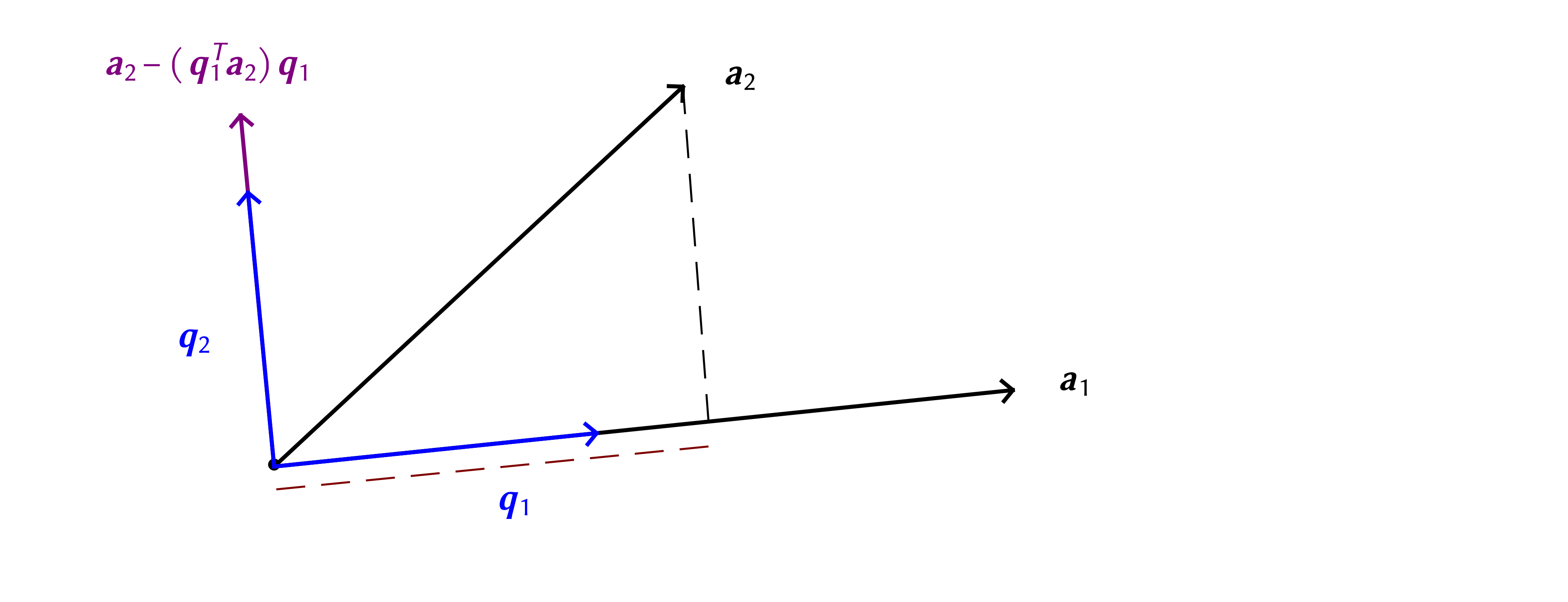
1.Projection 70

2.Gram-Schmidt 72

3. $Q R$ solution of linear algebra problems 73

3.1.Transformation of coordinates 73

3.2.General orthogonal bases 74

3.3.Least squares 75

Lecture 9: Reduced Systems 78

1.Projection of mappings 78

1.1.Reduced matrices 78

1.2.Dynamical system model reduction 79

2.Reduced bases 80

2.1.Correlation matrices 80

Correlation coefficient. 80

Patterns in data. 81

3.Stochastic systems - Karhunen-Loève theorem 82

Lecture 10: Square Linear Systems 83

1.Gaussian elimination and row echelon reduction 83

2. $L U$ -factorization 84

2.1.Example for $m = 3$ 84

2.2.General $m$ case 85

3.Matrix inverse 88

3.1.Gauss-Jordan algorithm 88

Lecture 11: $L U$ Algorithm Variants 89

1.Determinants 90

1.1.Cross product 93

2.Structured Matrices 93

3.Cholesky factorization of positive definite hermitian matrices 94

3.1.Symmetric matrices, hermitian matrices 94

3.2.Positive-definite matrices 95

3.3.Symmetric factorization of positive-definite hermitian matrices 95

Lecture 12: The Eigenvalue Problem 96

1.Definitions 96

1.1.Coordinate transformations 97

1.2.Paradigmatic eigenvalue problem solutions 97

1.3.Matrix eigendecomposition 99

1.4.Matrix properties from eigenvalues 101

1.5.Matrix eigendecomposition applications 101

2.Computation of the SVD 102

Lecture 13: Power Iterations 102

1.Reduction to triangular form 102

2.Power iteration for real symmetric matrices 103

2.1.The power iteration idea 104

2.2.Rayleigh quotient 104

2.3.Refining the power iteration idea 106

2. Scalar Function Approximation 109

Lecture 14: Interpolation 109

1.Function spaces 109

1.1.Infinite dimensional basis set 109

1.2.Alternatives to the concept of a basis 110

Fourier series. 111

Taylor series. 111

1.3.Common function spaces 111

2.Interpolation 112

2.1.Additive corrections 112

2.2.Polynomial interpolation 112

Monomial form of interpolating polynomial. 112

Lagrange form of interpolating polynomial. 114

Newton form of interpolating polynomial. 119

3.Interpolation error 121

3.1.Error minimization - Chebyshev polynomials 123

3.2.Best polynomial approximant 125

Lecture 15: Function and Derivative Interpolation 125

1.Interpolation in function and derivative values - Hermite interpolation 125

Monomial form of interpolating polynomial. 125

Lagrange form of interpolating polynomial. 127

Newton form of interpolating polynomial. 128

Lecture 16: Piecewise Interpolation 130

1.Splines 130

Constant splines (degree 0). 130

Linear splines (degree 1). 131

Quadratic splines (degree 2). 131

Cubic splines (degree 3). 132

2. $B$ -splines 133

Lecture 17: Spectral approximations 136

1.Trigonometric basis 136

1.1.Fourier series - Fast Fourier transform 136

1.2.Fast Fourier transform 137

1.3.Data-sparse matrices from Sturm-Liouville problems 137

2.Wavelet approximations 138

Lecture 18: Best Approximant 140

1.Best approximants 140

2.Two-norm approximants in Hilbert spaces 141

3.Inf-norm approximants 142

3. Linear Operator Approximation 145

Lecture 19: Derivative Approximation 145

1.Numerical differentiation based upon polynomial interpolation 145

Monomial basis. 145

Newton basis (finite difference calculus). 146

2.Taylor series methods 149

3.Numerical differentiation based upon piecewise polynomial interpolation 150

$B$ -spline basis. 150

Lecture 20: Quadrature 151

1.Numerical integration 151

Monomial basis. 151

Lagrange basis. 151

Moment method. 153

2.Gauss quadrature 154

Lecture 21: Ordinary Differential Equations - Single Step Methods 156

1.Ordinary differential equations 156

2.Differentiation operator approximation from polynomial interpolants 158

2.1.Euler forward scheme 158

2.2.Backward Euler scheme 158

2.3.Leapfrog scheme 159

Lecture 22: Ordinary Differential Equations - Multistep Methods 159

1.Adams-Bashforth and Adams-Moulton schemes 159

2.Simultaneous operator approximation - linear multistep methods 160

3.Consistency, convergence, stability 161

3.1.Model problem 161

3.2.Boundary locus method 162

4. Nonlinear Operator Approximation 165

Lecture 23: Nonlinear scalar operator equations 165

1.Root-finding algorithms 165

1.1.First-degree polynomial approximants 165

Secant method. 165

Newton-Raphson method. 166

1.2.Second-degree polynomial approximants 167

Halley's method. 167

2.Composite approximations 168

3.Fixed-point iteration 168

Lecture 24: Nonlinear Vector Operator Equations 170

1.Multivariate root-finding algorithms 170

2.Quasi-Newton methods 171

3.Gradient descent methods 172

Lecture 25: Introduction to nonlinear approximation 172

1.Historical analogue - operator calculus 173

1.1.Heavisde study of telgraphist equation 173

1.2.Development of mathematical theory of operator calculus 173

2.Basic approximation theory 174

2.1.Linear approximation example 174

2.2.Non-Linear approximation example 175

3.Nonlinear approximation by composition 176

Lecture 26: Data-Driven Nonlinear Approximation 176

1.Greedy bases 176

2.Artificial neural networks 176

3.Stochastic gradient descent 176

5. Differential Conservation Laws 177

Lecture 27: Differential Conservation Laws 177

1.The relevance of physics for scientific computation 177

2.Conservation laws 179

Banking example. 179

Local formulations. 181

3.Special forms of conservation laws 181

Second law of dynamics. 181

Advection equation. 181

Diffusion equation. 182

Combined effects. 182

Steady-state transport. 182

Separation of variables. 183

Lecture 28: Linear Operator Splitting 184

1.Poisson equation discretization 184

2.Matrix splitting iteration 186

3.Convergence analysis 186

Lecture 29: Gradient Descent Methods 191

1.Spatially dependent diffusivity 191

2.Steepest descent 193

3.Conjugate gradient 195

Lecture 30: Irregular Sparsity 196

1.Finite element discretization 196

2.Krylov methods, Arnoldi iteration 199

3.GMRES 201

Lecture 31: Incomplete Operator Decomposition 201

1.Finite difference Helmholtz equation 201

2.Arnoldi iteration 202

3.Lanczos iteration 204

Lecture 32: Bases for Incomplete Decomposition 205

1.Preconditioning 205

2.Multigrid 206

3.Random multigrid and stochastic descent 208

Lecture 33: Multiple Operators 209

1.Semi-discretization 209

2.Method of lines 210

3.Implicit-explicit methods 211

Lecture 34: Operator-Induced Bases 212

1.Spectral methods 212

2.Quasi-spectral methods 213

3.Fast transforms 215

Lecture 35: Nonlinear Operators 216

1.Advection equation 216

2.Convection equation 217

3.Discontinuous solutions 219

6. Integral Conservation Laws 221

III. Nonlinear Approximation 223

7. Computational Topology 227

8. Computational Geometry 229

9. Stochastic Differential Equations 231

10. Randomized Linear Algebra 233

Part I

Number Approximation

Most scientific disciplines introduce an idea of the amount of some entity or property of interest. Furthermore, the amount is usually combined with the concept of a number, an abstraction of the observation that the two sets {Mary, Jane, Tom} and {apple, plum, cherry} seem quite different, but we can match one distinct person to one distinct fruit as in {Maryplum, Janeapple, Tomcherry}. In contrast, we cannot do the same matching of distinct persons to a distinct color from the set {red, green}, and one of the colors must be shared between two persons. Formal definition of the concept of a number from the above observations is surprisingly difficult since it would be self-referential due to the apperance of the numbers “one” and “two”. Leaving this aside, the key concept is that of quantity of some property of interest that is expressed through a number.

Several types of numbers have been introduced in mathematics to express different types of quantities, and the following will be used throughout this text:

: The set of natural numbers, , infinite and countable, ;
: The set of integers, , infinite and countable;
: The set of rational numbers , infinite and countable;
: The set of real numbers, infinite, not countable, can be ordered;
: The set of complex numbers, , infinite, not countable, cannot be ordered.

These sets of numbers form a hierarchy, with . The size of a set of numbers is an important aspect of its utility in describing natural phenomena. The set has three elements, and its size is defined by the cardinal number, . The sets have an infinite number of elements, but the relation

z = {\begin{cases} - n / 2 & for n even \\ (n + 1) / 2 & for n odd \end{cases} .

defines a one-to-one correspondence between and , so these sets are of the same size denoted by the transfinite number (aleph-zero). The rationals can also be placed into a one-to-one correspondence with , hence

| ℕ | = | ℤ | = | ℚ | = ℵ_{0} .

In contrast there is no one-to-one mapping of the reals to the naturals, and the cardinality of the reals is (Fraktur-script c). Georg Cantor established set theory and introduced a proof technique known as the diagonal argument to show that . Intuitively, there are exponentially more reals than naturals.

One of the foundations of the scientific method is quantification, ascribing numbers to phenomena of interest. To exemplify the utility of different types of number to describe natural phenomena, consider common salt (sodium chloride, Fig. ) which has the chemical formula NaCl with the sodium ions () and chloride ions () spatially organized in a cubic lattice, with an edge length Å (1 Å = m) between atoms of the same type. Setting the origin of a Cartesian coordinate system at a sodium atom, the position of some atom within the lattice is

(x, y, z) = (i \frac{a}{2}, j \frac{a}{2}, k \frac{a}{2}) .

Sodium atoms are found positions where is even, while chloride atoms are found at positions where is odd. The Cartesian coordinates describe some arbitrary position in space, which is conceptualized as a continuum and placed into one-to-one correspondence with . A particular lattice position can be specified simply through a label consisting of three integers . The position can be recovered through a scaling operation

(x, y, z) = \frac{a}{2} (i, j, k),

and the number that modifies the length scale from to , it is called a scalar.

A computer has a finite amount of memory, hence cannot represent all numbers, but rather subsets of the above number sets. Current digital computers internally use numbers represented through binary digits, or bits. Many computer number types are defined for specific purposes, and are often encountered in applications such as image representation or digital data acquisition. Here are the main types.

Subsets of

The number types uint8, uint16, uint32, uint64 represent subsets of the natural numbers (unsigned integers) using 8, 16, 32, 64 bits respectively. An unsigned integer with bits can store a natural number in the range from to . Two arbitrary natural numbers, written as can be added and will give another natural number, . In contrast, addition of computer unsigned integers is only defined within the specific range to . If , the result might be displayed as the maximum possible value or as .

Subsets of

The number types int8, int16, int32, int64 represent subsets of the integers. One bit is used to store the sign of the number, so the subset of that can be represented is from to .

Subsets of

Computers approximate the real numbers through the set of floating point numbers. Floating point numbers that use bits are known as single precision, while those that use are double precision. A floating point number is stored internally as where , are bits within the mantissa of length , and , are bits within the exponent, along with signs for each. The default number type is usually double precision, more concisely referred to Float64. Common irrational constants such as , are predefined as irrationals and casting to Float64 or Float32 gives floating point approximation. Unicode notation is recognized. Specification of a decimal point indicates a floating point number; its absence indicates an integer.

The approximation of the reals by the floats is characterized by: floatmax(), the largest float, floatmin the smallest positive float, and eps() known as machine epsilon. Machine epsilon highlights the differences between floating point and real numbers since it may be informally defined as the smallest number of form that satisfies . If of course implies , but floating points exhibit “granularity”, in the sense that over a unit interval there are small steps that are indistinguishable from zero due to the finite number of bits available for a float leading to being indistiguishable from 1, and the apparently endless loop shown below actually terminates.

The granularity of double precision expressed by machine epsilon is sufficient to represent natural phenomena, and floating point errors can usually be kept under control,

Keep in mind that perfect accuracy is a mathematical abstraction, not encountered in nature. In fields such as sociology or psychology 3 digits of accuracy are excellent, in mechanical engineering this might increase to 6 digits, or in electronic engineering to 8 digits. The most precisely known physical constant is the Rydberg constant known to 12 digits, hence a mathematical statement such as

x = 2.6309283450461248350319486319845

is unlikely to have any real significance, while

x = 2.631 \pm 0.0005

is much more informative.

Within the reals certain operations are undefined such as . Special float constants are defined to handle such situations: Inf is a float meant to represent infinity, and NaN (“not a number”) is meant to represent an undefinable result of an arithmetic operation.

Complex numbers are specified by two reals, in Cartesian form as , or in polar form as , , . The computer type complex is similarly defined from two floats and the additional constant I is defined to represent . Functions are available to obtain the real and imaginary parts within the Cartesian form, or the absolute value and argument of the polar form.

The reals form an algebraic structure known as a field . The set of floats together with floating point addition and multiplication are denoted as . Operations with floats do not have the same properties as the reals, but are assumed to have a relative error bounded by machine epsilon

\forall x, y \in ℝ, | \frac{fl (x) ⊛ fl (y) - x * y}{x * y} | ⩽ ϵ, (⊛, *) \in {(\oplus, +), (⊙, \cdot)},

where is the floating point representation of . The above is restated

fl (x) ⊛ fl (y) = (x * y) (1 + ε), | ε | ⩽ ϵ,

and accepted as an axiom for use in error analysis involving floating point arithmetic. Computer number sets are a first example of approximation: replacing some complicated object with a simpler one. It is one of the key mathematical ideas studied throughout this text.

Care should be exercised about the cummulative effect of many floating point operations. An informative example is offered by Zeno's paradox of motion, that purports that fleet-footed Achilles could never overcome an initial head start of given to the lethargic Tortoise since, as stated by Aristotle:

The above is often formulated by considering that the first half of the initial head start must be overcome, then another half and so on. The distance traversed after such steps is

D_{N} = 1 + \frac{1}{2} + \dots + \frac{1}{2^{N}} = \frac{1 - {(1 / 2)}^{N + 1}}{1 - (1 / 2)} = 2 [1 - {(1 / 2)}^{N + 1}] < 2 .

Calculus resolves the paradox by rigorous definition of the limit and definition of velocity as , , .

Undertake a numerical invesigation and consider two scenarios, with increasing or decreasing step sizes

D_{N} = 1 + \frac{1}{2} + \dots + \frac{1}{2^{N}}, C_{N} = \frac{1}{2^{N}} + \frac{1}{2^{N - 1}} + \dots + 1 .

In associativity ensures .

Irrespective of the value for , in floating point arithmetic. Recall however that computers use binary representations internally, so division by powers of two might have unique features (indeed, it corresponds to a bit shift operation). Try subdividing the head start by a different number, perhaps to get an “irrational” numerical investigation of Zeno's paradox of motion. Define now the distance traversed by step sizes that are scaled by starting from one to , traversed by step sizes scaled by starting from

S_{N} = 1 + \frac{1}{π} + \frac{1}{π^{2}} + \dots + \frac{1}{π^{N}}, T_{N} = \frac{1}{π^{N}} + \frac{1}{π^{N - 1}} + \dots + 1 .

Again, in the reals the above two expressions are equal, , but this is no longer verified computationally for all , not even within a tolerance of machine epsilon.

This example gives a first glimpse of the steps that need to be carried out in addition to mathematical analysis to fully characterize an algorithm. Since , a natural question is whether one is more accurate than the other. For some arbitrary ratio , the exact value is known

E_{N} = \frac{1 - {(1 / a)}^{N + 1}}{1 - (1 / a)},

and can be used to evaluate the errors , .

Carrying out the computations leads to results in Fig. .

Note that errors are about the size of machine epsilon for , but are zero for , it seems that the summation ordering gives the exact value. A bit of reflection reinforces this interpretation: first adding small quantities allows for carry over digits to be accounted for.

This example is instructive beyond the immediate adage of “add small quantities first”. It highlights the blend of empirical and analytical approaches that is prevalent in scientific computing.

Single values given by some algorithm are of little value in the practice of scientific computing. The main goal is the construction of a sequence of approximations that enables assessment of the quality of an approximation. Recall from calculus that converges to if can be made as small as desired for all beyond some threshold. In precise mathematical language this is stated through:

Though it might seem natural to require a sequence of approximations to converge to an exact solution

{lim}_{n \to \infty} x_{n} = x,

such a condition is problematic on multiple counts:

the exact solution is rarely known;
the best approximation might be achieved for some finite range , rather than in the limit.

Both situations arise when approximating numbers and serve as useful reference points when considering approximation other types of mathematical objects such as functions. For example, the number is readily defined in geometric terms as the ratio of circle circumference to diameter, but can only be approximately expressed by a rational number, e.g., . The exact value of is only obtained as the limit of an infinite number of operations with rationals. There are many such infinite representations, one of which is the Leibniz series

\frac{π}{4} = 1 - \frac{1}{3} + \frac{1}{5} - \frac{1}{7} + \frac{1}{9} - \dots . .

No finite term

L_{n} = \sum_{k = 0}^{n} \frac{{(- 1)}^{k}}{2 k + 1}

of the above Leibniz series equals , i.e.,

\exists n \in ℕ such that L_{n} = π / 4 .

Rather, the Leibniz series should be understood as an algorithm, i.e., a sequence of elementary operations that leads to succesively more accurate approximations of

{lim}_{n \to \infty} L_{n} = π / 4 .

Complex analysis provides a convergence proof starting from properties of the function

\frac{d}{d z} \arctan (z) = \frac{1}{1 + z^{2}} \Rightarrow \frac{π}{4} = \arctan (1) - \arctan (0) = \int_{0}^{1} \frac{d z}{1 + z^{2}} .

For the sequence of partial sums of a geometric series converges uniformly

\sum_{k = 0}^{\infty} {(- z^{2})}^{k} = {lim}_{n \to \infty} \frac{1 - {(- z^{2})}^{n}}{1 - (- z^{2})} = \frac{1}{1 + z^{2}},

and can be integrated term by term to give

\frac{π}{4} = \int_{0}^{1} \sum_{k = 0}^{\infty} {(- z^{2})}^{k} d z = \sum_{k = 0}^{\infty} \int_{0}^{1} {(- z^{2})}^{k} d z = \sum_{k = 0}^{\infty} \frac{{(- 1)}^{k}}{2 k + 1} .

This elegant result does not address however the points raised above: if were not known, how could the convergence of the sequence be assessed? A simple numerical experiment indicates that the familiar value of is only recovered for large , with 10000 terms insufficient to ensure five significant digits.

Instead of evaluating distance to an unknown limit, as in , one could evaluate if terms get closer to one another as in , a condition that can readily be checked in an algorithm.

Note that the distance between any two terms after the threshold must be smaller than an arbitrary tolerance . For example the sequence is not a Cauchy sequence even though the distance between successive terms can be made arbitrarily small

a_{n + 1} - a_{n} = \sqrt{n + 1} - \sqrt{n} = \frac{(\sqrt{n + 1} - \sqrt{n}) (\sqrt{n + 1} + \sqrt{n})}{\sqrt{n + 1} + \sqrt{n}} = \frac{1}{\sqrt{n + 1} + \sqrt{n}} < \frac{1}{2 \sqrt{n}} .

Verification of decreasing successive distance is therefore a necessary but not sufficient condition to assess whether a sequence is a Cauchy sequence. Furthermore, the distance between successive iterates is not necessarily an indication of the distance to the limit. Reprising the Leibniz example, successive terms can be further apart than the distance to the limit, though terms separated by 2 are closer than the distance to the limit (a consequence of the alternating Leibniz series signs)

Another question is whether a Cauchy sequence is itself convergent. For sequences of reals this is true, but the Leibniz sequence furnishes a counterexample since it contains rationals and converges to an irrational. Such aspects that arise in number approximation sequences become even more important when considering approximation sequences composed of vectors or functions.

Consideration of floating point arithmetic indicates adaptation of the mathematical concept of convergence is required in scientific computation. Recall that machine epsilon is that largest number such that is true, and characterizes the granularity of the floating point system. A reasonable adaptation of the notion of convergence might be:

What emerges is the need to consider a degree of uncertainty in an approximating sequence. If the uncertainty can be bounded to the intrinsic granularity of the number system, a good approximation is obtained.

The problem of approximating numbers uncovers generic aspects of scientific computing:

different models of some phenomenon are possible and it is necessary to establish correspondence between models and of a model to theory;
scientific computation seeks to establish viable approximation techniques for the mathematical objects that arise in models;
correspondence of a model to theory is established through properties of approximation sequences, not single results of a particular approximation technique;
physical limitations of computer memory require revisiting of mathematical concepts to characterize approximation sequence behavior, and impart a stochastic aspect to approximation techniques;
computational experiments are a key aspect, giving an empirical aspect to scientific computing that is not found in deductive or analytical mathematics.

The objective of scientific computation is to solve some problem by constructing a sequence of approximations . The condition suggested by mathematical analysis would be , with . As already seen in the Leibniz series approximation of , acceptable accuracy might only be obtained for large . Since could be an arbitrarily complex mathematical object, such slowly converging approximating sequences are of little practical interest. Scientific computing seeks approximations of the solution with rapidly decreasing error. This change of viewpoint with respect to analysis is embodied in the concepts of rate and order of convergence.

As previously discussed, the above definition is of limited utility since:

The solution is unknown;

The limit is impractical to attain.

Sequences converge faster for higher order or lower rate . A more useful approach is to determine estimates of the rate and order of convergence over some range of iterations that are sufficiently accurate. Rewriting () as

{lim}_{n \to \infty} (| x_{n + 1} - x | - r {| x_{n} - x |}^{p}) = 0,

suggests introducing the distance between successive iterates , and considering the condition

| d_{n + 1} - s d_{n}^{q} | small for large n .

As an example, consider the derivative of at , as given by the calculus definition

g (x_{0}) = f^{'} (x_{0}) = {lim}_{h \to 0} \frac{f (x_{0} + h) - f (x_{0})}{h},

and construct a sequence of approximations

g_{n} = \frac{f_{n} - f (0)}{h_{n}}, f_{n} = f (h_{n}), h_{n} = 2^{- n} .

Start with a numerical experiment, and compute the sequence .

Investigation of the numerical results indicates increasing accuracy in the estimate of , with decreasing step size . The distance between successive approximation sequence terms also decreases. It is more intuitive to analyze convergence behavior through a plot rather than a numerical table.

The intent of the rate and order of approximation definitions is to state that the distance between successive terms behaves as

d_{n + 1} ≅ s d_{n}^{q},

in the hope that this is a Cauchy sequence, and successively closer terms actually indicate convergence. The convergence parameters can be isolated by taking logarithms, leading to a linear dependence

c_{n + 1} ≅ q c_{n} + \log s .

Subtraction of successive terms gives , leading to an average slope estimate

q ≅ \frac{1}{N - 3} \sum_{n = 3}^{N - 1} \frac{c_{n} - c_{n - 1}}{c_{n - 1} - c_{n - 2}}

The above computations indicate , known as linear convergence. Figure b shows the common practice of depicting guide lines of slope 1 (black) and slope 2 (green) to visually ascertain the rate of convergence. Once the order of approximation is determined, the rate of aproximation is estimated from

\log s ≅ \frac{1}{N - 2} \sum_{n = 2}^{N - 1} (c_{n} - q c_{n - 1}) .

The above results suggest successive approximants become closer spaced according to

d_{n} ≅ 0.124 d_{n - 1}

Repeat the above experiment at , where , and using a different approximation of the derivative

g_{n} = \frac{f (\ln 2 + h_{n}) - f (\ln 2 - h_{n})}{2 h_{n}} .

For this experiment, in addition to the rate and order of approximation , also determine the rate and order of convergence using

b_{n} = | g_{n} - g (π / 4) |, b_{n + 1} ≅ r b_{n}^{p}, a_{n} = \log b_{n}, a_{n + 1} = p a_{n} + \log r .

Given some approximation sequence , , with solution of problem , it is of interest to construct a more rapidly convergent sequence , . Knowledge of the order of convergence can be used to achieve this purpose by writing

and taking the ratio to obtain

For , the above is a polynomial equation of degree that can be solved to obtain . The heuristic approximation () suggests a new approximation of the exact limit obtained by solving ().

One of the widely used acceleration techniques was published by Aitken (1926, but had been in use since Medieval times) for in which case () gives

x_{n} x_{n - 2} - (x_{n} + x_{n - 2}) x = x_{n - 1}^{2} - 2 x_{n - 1} x \Rightarrow x = \frac{x_{n} x_{n - 2} - x_{n - 1}^{2}}{x_{n} - 2 x_{n - 1} + x_{n - 2}} .

The above suggests that starting from , the sequence with

a_{n} = \frac{x_{n} x_{n - 2} - x_{n - 1}^{2}}{x_{n} - 2 x_{n - 1} + x_{n - 2}} = x_{n} - \frac{{(x_{n} - x_{n - 1})}^{2}}{x_{n} - 2 x_{n - 1} + x_{n - 2}},

might converge faster towards the limit. Investigate by revisiting the numerical experiment on approximation of the derivative of at , using

g_{n} = \frac{f_{n} - f (0)}{h_{n}}, f_{n} = f (h_{n}), h_{n} = 2^{- n} .

Analysis reinforces the above numerical experiment. First-order convergence implies the distance to the limit decreases during iteration as

Several approaches may be used in construction of an approximating sequence . The approaches exemplified below for , can be generalized when is some other type of mathematical object.

Returning to the Leibniz series

\frac{π}{4} = 1 - \frac{1}{3} + \frac{1}{5} - \frac{1}{7} + \frac{1}{9} - \dots .,

the sequence of approximations is with general term

L_{n} = \sum_{k = 0}^{n} \frac{{(- 1)}^{k}}{2 k + 1} .

Note that successive terms are obtained by an additive correction

L_{n} = L_{n - 1} + \frac{{(- 1)}^{n}}{2 n + 1}, L_{n} \to \frac{π}{4} .

Another example, again giving an approximation of is the Srinivasa Ramanujan series

R_{n} = \frac{2 \sqrt{2}}{9801} \sum_{k = 0}^{n} \frac{(4 k)! (1103 + 26390 k)}{{(k!)}^{4} 396^{4 k}}, {lim}_{n \to \infty} R_{n} = \frac{1}{π},

that can be used to obtain many digits of accuracy with just a few terms.

An example of the generalization of this approach is the Taylor series of a function. For example, the familiar sine power series

\sin x = x - \frac{x^{3}}{3!} + \frac{x^{5}}{5!} - \dots,

is analogous, but with rationals now replaced by monomials, and the limit is now a function . The general term is

T_{n} (x) = \sum_{k = 0}^{n} \frac{{(- 1)}^{k} x^{2 k + 1}}{(2 k + 1)!},

and the same type of additive correction appears, this time for functions,

T_{n} (x) = T_{n - 1} (x) + \frac{{(- 1)}^{n} x^{2 n + 1}}{(2 n + 1)!}, T_{n} (x) \to \sin x .

Approximating sequences need not be constructed by adding a correction. Consider the approximation of given by Wallis's product (1656)

S_{n} = (\frac{2}{1} \cdot \frac{2}{3}) \cdot (\frac{4}{3} \cdot \frac{4}{5}) \cdot (\frac{6}{5} \cdot \frac{6}{7}) \dots, S_{n} = \prod_{k = 1}^{n} \frac{4 k^{2}}{4 k^{2} - 1}, S_{n} \to \frac{π}{2},

for which

S_{n} = S_{n - 1} \cdot (\frac{4 n^{2}}{4 n^{2} - 1}) .

Another famous example is the Viète formula from 1593

\frac{2}{π} = \frac{\sqrt{2}}{2} \cdot \frac{\sqrt{2 + \sqrt{2}}}{2} \cdot \frac{\sqrt{2 + \sqrt{2 + \sqrt{2}}}}{2} \cdot \dots, V_{n} = \prod_{k = 1}^{n} \frac{\overset{k}{j = 1} \sqrt[2]{2}}{2}

in which the correction is multiplicative with numerators given by nested radicals. Similar to the symbol for addition, and the symbol for multiplication, the N symbol is used to denote nested radicals

\overset{k}{j = 1} \sqrt[b_{}]{a_{j}} = \sqrt[b_{1}]{a_{1} + \sqrt[b_{2}]{a_{2} + \sqrt[b_{3}]{a_{3} + \dots + \sqrt[b_{k}]{a_{k}}}}} .

In the case of the Viète formula, , for all .

Yet another alternative is that of continued fractions, with one possible approximation of given by

A notation is introduced for continued fractions using the symbol

F_{n} = b_{0} + \overset{n}{k = 1} \frac{a_{k}}{b_{k}} = b_{0} + \frac{a_{1}}{b_{1} +} .

Using this notation, the sequences arising in the continued fraction representation of are , chosen as for , and for .

π = {lim}_{n \to \infty} (6 + \overset{n}{k = 1} \frac{{(2 k - 1)}^{2}}{6}) .

The above correction techniques used arithmetic operations. The repeated radical coefficients in the Viète formula suggest consideration of repeated composition of arbitrary functions to construct the approximant

insect

T_{n} = t_{0} \circ t_{1} \circ \dots \circ t_{n} = ⊙_{k = 0}^{n} t_{k} .

This is now a general framework, in which all of the preceeding correction approaches can be expressed. For example, the continued fraction formula () is recovered through the functions

t_{0} (z) = 6 + z, t_{1} (z) = \frac{1}{6 + z}, \dots, t_{k} (z) = \frac{{(2 k - 1)}^{2}}{6 + z},

and evaluation of the composite function at

F_{n} = T_{n} (0) .

This general framework is of significant current interest since such composition of nonlinear functions is the basis of deep neural network approximations.

The cornerstone of scientific computing is construction of approximating sequences.
The problem of number approximation leads to definition of concepts and techniques that can be extended to more complex mathematical objects.
A primary objective is the construction of efficient approximating sequences, with efficiency characterized through concepts such as order and speed of convergence.
Though often enforced analytically, limiting behavior of the sequence is of secondary interest. As seen in the approximation of a derivative, the approximating sequence might diverge, yet give satisfactory answers for some range of indices.
Though by far the most widely studied and used approach to approximation, additive corrections are not the only possibility.
Alternative correction techniques include: multiplication, continued fractions, or repeated function composition.
Repeated composition of functions is used in constructing deep neural network approximants.

In general, mathematical problems can be thought of as mappings from some set of inputs to some set of outputs . The mapping is often carried out through a function , i.e., a procedure that associates a single to some input

f : X \to Y, y = f (x), x \overset{f}{\to} y

Examples:

Note that the specification of a mathematical problem requires definition of the triplet .

Once a problem is specified, the natural question is to ascertain whether a solution is possible. Generally, simple affirmation of the existence of a solution is the objective of some field of mathematics (e.g., analysis, functional analysis). From the point of view of science, an essential question is not only existence but also:

how does the output change if changes?
what are the constructive methods to approximate ?

The above general definition of a mathematical problem must be refined in order to assess magnitude of changes in inputs or outputs. A first step is to introduce some structure in the input and output sets . Using these sets, vector spaces are constructed, consisting of a set of vectors , a set of scalars , an addition operation , and a scaling operation . The vector space is often referred to simply by its set of vectors , when the set of scalars, addition operation, and scaling operation are self-evident in context.

Formally,a vector space is defined by a set whose elements satisfy certain scaling and addition properties, denoted all together by the 4-tuple . The first element the 4-tuple is a set whose elements are called vectors. The second element is a set of scalars, and the third is the vector addition operation. The last is the scaling operation, seen as multiplication of a vector by a scalar. The vector addition and scaling operations must satisfy rules suggested by positions or forces in three-dimensional space, which are listed in Table . In particular, a vector space requires definition of two distinguished elements: the zero vector , and the identity scalar element .

A first step is quantification of the changes in input or output, assumed to have the structure of a vector space, .

The ratio of changes in output to changes in input is the absolute condition number of a problem.

To avoid influence of choice of reference unit, the relative condition number is also introduced.

In scientific computation, the mathematical problem is approximated by an algorithm , in which is assumed to be computable, and are vector spaces that approximate . As a first step in characterizing how well the algorithm approximates the problem , consider that and , i.e., there is no error in representation of the domain and codomain.

The above condition is also denoted as

Algorithms should not catastrophically increase input errors. This is quantified in the concept of stability.

The above states that the relative error in the output should be on the order of machine epsilon if the relative in the input is of order machine epsilon. Note that the constants in the order statements are usually different from one another, ,

Backward stability asserts that the result of the algorithm on exact input data is the same as the solution to the mathematical problem for nearby data (with distance on order of machine epsilon).

Mathematical problems are stated as functions from a set of inputs to a set of outputs ,
The difficulty of a mathematical problem is assessed by measuring the effect of changes in input
To quantify changes in inputs and outputs, the framework of a normed vector space is introduced
The ratio of norm of output change to norm of input change is the absolute condition number of a problem
$\hat{κ} = {lim}_{ε \to 0} {sup}_{|| δ x || ⩽ ε} \frac{|| f (x + δ x) - f (x) ||}{|| δ x ||}$
Algorithms are constructive approximations of mathemtical problems . The accuracy of an algorithm is assessed by comparison of the algorithm output to that of the mathematical problem through absolute error and relative error
$e = || \tilde{f} (x) - f (x) ||, ε = \frac{|| \tilde{f} (x) - f (x) ||}{|| f (x) ||}$
The tendency of an algorithm to amplify pertubations of input is assessed by the concept of stability
Algorithms that do not amplify relative changes in input of the size of machine precision are forward stable.
Algorithms that compute the exact result of a mathematical problem for changes in put of the size of machine precision are backward stable.

Part II

Linear Approximation

Chapter 1
Linear Algebra

The definition from Table 1 of a vector space reflects everyday experience with vectors in Euclidean geometry, and it is common to refer to such vectors by descriptions in a Cartesian coordinate system. For example, a position vector within the plane can be referred through the pair of coordinates . This intuitive understanding can be made precise through the definition of a vector space , called the real 2-space. Vectors within are elements of , meaning that a vector is specified through two real numbers, . Addition of two vectors, , is defined by addition of coordinates . Scaling by scalar is defined by . Similarly, consideration of position vectors in three-dimensional space leads to the definition of the , or more generally a real -space , , .

Note however that there is no mention of coordinates in the definition of a vector space as can be seen from the list of properties in Table 1. The intent of such a definition is to highlight that besides position vectors, many other mathematical objects follow the same rules. As an example, consider the set of all continuous functions , with function addition defined by the sum at each argument , and scaling by defined as . Read this as: “given two continuous functions and , the function is defined by stating that its value for argument is the sum of the two real numbers and ”. Similarly: “given a continuous function , the function is defined by stating that its value for argument is the product of the real numbers and ”. Under such definitions is a vector space, but quite different from . Nonetheless, the fact that both and are vector spaces can be used to obtain insight into the behavior of continuous functions from Euclidean vectors, and vice versa. This correspondence principle between discrete and continuous formulations is a recurring theme in scientific computation.

Since the real spaces play such an important role in themselves and as a guide to other vector spaces, familiarity with vector operations in is necessary to fully appreciate the utility of linear algebra to a wide range of applications. Following the usage in geometry and physics, the real numbers that specify a vector are called the components of . The one-to-one correspondence between a vector and its components , is by convention taken to define an equality relationship,

with the components arranged vertically and enclosed in square brackets. Given two vectors , and a scalar , vector addition and scaling are defined in by real number addition and multiplication of components

The vector space is defined using the real numbers as the set of scalars, and constructing vectors by grouping together scalars, but this approach can be extended to any set of scalars , leading to the definition of the vector spaces . These will often be referred to as -vector space of scalars, signifying that the set of vectors is .

To aid in visual recognition of vectors, the following notation conventions are introduced:

vectors are denoted by lower-case bold Latin letters: ;

scalars are denoted by normal face Latin or Greek letters: ;

the components of a vector are denoted by the corresponding normal face with subscripts as in equation ();

related sets of vectors are denoted by indexed bold Latin letters: .

Instead of the vertical placement or components into one column, the components of could have been placed horizontally in one row , that contains the same data, differently organized. By convention vertical placement of vector components is the preferred organization, and shall denote a column vector henceforth. A transpose operation denoted by a superscript is introduced to relate the two representations

and is the notation used to denote a row vector.

Addition of real vectors defines another vector . The components of are the sums of the corresponding components of and , , for . Addition of vectors with different number of components is not defined, and attempting to add such vectors produces an error. Such vectors with different number of components are called incompatible, while vectors with the same number of components are said to be compatible. Scaling of by defines a vector , whose components are , for .

The vectors used in applications usually have a large number of components, , and it is important to become proficient in their manipulation. Previous examples defined vectors by explicit listing of their components. This is impractical for large , and support is provided for automated generation for often-encountered situations. First, observe that Table 1 mentions one distinguished vector, the zero element that is a member of any vector space . The zero vector of a real vector space is a column vector with components, all of which are zero, and a mathematical convention for specifying this vector is . This notation specifies that transpose of the zero vector is the row vector with zero components, also written through explicit indexing of each component as , for . Keep in mind that the zero vector and the zero scalar are different mathematical objects.

The ellipsis symbol in the mathematical notation is transcribed in Julia by the notion of a range, with 1:m denoting all the integers starting from to , organized as a row vector. The notation is extended to allow for strides different from one, and the mathematical ellipsis is denoted as m:-1:1. In general r:s:t denotes the set of numbers with , and real numbers and a natural number, , . If there is no natural number such that , an empty vector with no components is returned.

The expression expresses the idea of scaling vectors within a set and subsequent addition to form a new vector . The matrix groups these vectors together in a single entity, and the scaling factors are the components of the vector . To bring all these concepts together it is natural to consider the notation

as a generalization of the scalar expression . It is clear what the operation should signify: it should capture the vector scaling and subsequent vector addition . A specific meaning is now ascribed to by identifying two definitions to one another.

Repeateadly stating “vector scaling and subsequent vector addition” is unwieldy, so a special term is introduced for some given set of vectors .

Similar to the grouping of unit vectors into the identity matrix , a more concise way of referring to arbitrary vectors from the same vector space is the matrix . Combining these observations leads to the definition of a matrix-vector product.

Consider a simple example that leads to a common linear algebra problem: decomposition of forces in the plane along two directions. Suppose a force is given in terms of components along the Cartesian -axes, , as expressed by the matrix-vector multiplication Note that the same force could be obtained by linear combination of other vectors, for instance the normal and tangential components of the force applied on an inclined plane with angle , , as in Figure . This defines an alternate reference system for the problem. The unit vectors along these directions are

and can be combined into a matrix . The value of the components are the scaling factors and can be combined into a vector . The same force must result irrespective of whether its components are given along the Cartesian axes or the inclined plane directions leading to the equality

Interpret equation () to state that the vector could be obtained either as a linear combination of , , or as a linear combination of the columns of , . Of course the simpler description seems to be for which the components are already known. But this is only due to an arbitrary choice made by a human observer to define the force in terms of horizontal and vertical components. The problem itself suggests that the tangential and normal components are more relevant; for instance a friction force would be evaluated as a scaling of the normal force.

Linear combinations in a real space can suggest properties or approximations of more complex objects such as continuous functions. Let denote the vector space of continuous functions that are periodic on the interval , . Recall that vector addition is defined by , and scaling by , for , . Familiar functions within this vector space are , with , and these can be recognized to intrinsically represent periodicity on , a role analogous to the normal and tangential directions in the inclined plane example. Define now another periodic function by repeating the values from the interval on all intervals , for . The function is not given in terms of the “naturally” periodic functions , , but could it thus be expressed? This can be stated as seeking a linear combination as studied in Fourier analysis. The coefficients could be determined from an analytical formula involving calculus operations but we'll seek an approximation using a linear combination of terms

b (t) ≅ \sum_{k = 1}^{n} x_{k} \sin (k t), A (t) = [\begin{array}{llll} \sin (t) & \sin (2 t) & \dots & \sin (n t) \end{array}], A : ℝ \to ℝ^{n} .

Organize this as a matrix vector product , with

A (𝒕) = [\begin{array}{llll} \sin (𝒕) & \sin (2 𝒕) & \dots & \sin (n 𝒕) \end{array}], 𝒙 = {[\begin{array}{llll} x_{1} & x_{2} & \dots & x_{n} \end{array}]}^{T} \in ℝ^{n} .

The idea is to sample the column vectors of at the components of the vector , , , . Let , and , denote the so-sampled functions leading to the definition of a vector and a matrix . There are coefficients available to scale the column vectors of , and has components. For it is generally not possible to find such that would exactly equal , but as seen later the condition to be as close as possible to leads to a well defined solution procedure. This is known as a least squares problem and is automatically applied in the x=A\b instruction when the matrix A is not square. As seen in the following numerical experiment and Figure , the approximation is excellent and the information conveyed by samples of is now much more efficiently stored in the form chosen for the columns of and the scaling coefficients that are the components of .

A widely used framework for constructing additive approximations is the vector space algebraic space structure in which scaling and addition operations are defined
In a vector space linear combinations are used to construct more complicated objects from simpler ones
$𝒃 = 𝑨 𝒙 = x_{1} 𝒂_{1} + \dots + x_{n} 𝒂_{n}$

A general procedure to relate input values from set to output values from set is to first construct the set of all possible instances of and , which is the Cartesian product of with , denoted as . Usually only some associations of inputs to outputs are of interest leading to the following definition.

Associating an output to an input is also useful, leading to the definition of an inverse relation as , . Note that an inverse exists for any relation, and the inverse of an inverse is the original relation, .

Many types of relations are defined in mathematics and encountered in linear algebra. A commonly encountered type of relationship is from a set onto itself, known as a homogeneous relation. For homogeneous relations , it is common to replace the set membership notation to state that is in relationship with , with a binary operator notation . Familiar examples include the equality and less than relationships between reals, , in which is replaced by , and is replaced by . The equality relationship is its own inverse, and the inverse of the less than relationship is the greater than relation , , . Homogeneous relations are classified according to the following criteria.

Reflection: Relation is reflexive if for any . The equality relation is reflexive, , the less than relation is not, .
Symmetry: Relation is symmetric if implies that , . The equality relation is symmetric, , the less than relation is not, .
Anti-symmetry: Relation is anti-symmetric if for , then . The less than relation is antisymmetric, .
Transitivity: Relation is transitive if and implies . for any . The equality relation is transitive, , as is the less than relation , .

Certain combinations of properties often arise. A homogeneous relation that is reflexive, symmetric, and transitive is said to be an equivalence relation. Equivalence relations include equality among the reals, or congruence among triangles. A homogeneous relation that is reflexive, anti-symmetric and transitive is a partial order relation, such as the less than or equal relation between reals. Finally, a homogeneous relation that is anti-symmetric and transitive is an order relation, such as the less than relation between reals.

Functions between sets and are a specific type of relationship that often arise in science. For a given input , theories that predict a single possible output are of particular scientific interest.

The above intuitive definition can be transcribed in precise mathematical terms as is a function if and implies . Since it's a particular kind of relation, a function is a triplet of sets , but with a special, common notation to denote the triplet by , with and the property that . The set is the domain and the set is the codomain of the function . The value from the domain is the argument of the function associated with the function value . The function value is said to be returned by evaluation .

As seen previously, a Euclidean space can be used to suggest properties of more complex spaces such as the vector space of continuous functions . A construct that will be often used is to interpret a vector within as a function, since with components also defines a function , with values . As the number of components grows the function can provide better approximations of some continuous function through the function values at distinct sample points .

The above function examples are all defined on a domain of scalars or naturals and returned scalar values. Within linear algebra the particular interest is on functions defined on sets of vectors from some vector space that return either scalars , or vectors from some other vector space , . The codomain of a vector-valued function might be the same set of vectors as its domain, . The fundamental operation within linear algebra is the linear combination with , . A key aspect is to characterize how a function behaves when given a linear combination as its argument, for instance or

Consider first the case of a function defined on a set of vectors that returns a scalar value. These can be interpreted as labels attached to a vector, and are very often encountered in applications from natural phenomena or data analysis.

Many different functionals may be defined on a vector space , and an insightful alternative description is provided by considering the set of all linear functionals, that will be denoted as . These can be organized into another vector space with vector addition of linear functionals and scaling by defined by

As is often the case, the above abstract definition can better be understood by reference to the familiar case of Euclidean space. Consider , the set of vectors in the plane with the position vector from the origin to point in the plane with coordinates . One functional from the dual space is , i.e., taking the second coordinate of the position vector. The linearity property is readily verified. For , ,

f_{2} (a 𝒙 + b 𝒚) = a x_{2} + b y_{2} = a f_{2} (𝒙) + b f_{2} (𝒚) .

Given some constant value , the curves within the plane defined by are called the contour lines or level sets of . Several contour lines and position vectors are shown in Figure . The utility of functionals and dual spaces can be shown by considering a simple example from physics. Assume that is the height above ground level and a vector is the displacement of a body of mass in a gravitational field. The mechanical work done to lift the body from ground level to height is with the gravitational acceleration. The mechanical work is the same for all displacements that satisfy the equation . The work expressed in units can be interpreted as the number of contour lines intersected by the displacement vector . This concept of duality between vectors and scalar-valued functionals arises throughout mathematics, the physical and social sciences and in data science. The term “duality” itself comes from geometry. A point in with coordinates can be defined either as the end-point of the position vector , or as the intersection of the contour lines of two functionals and . Either geometric description works equally well in specifying the position of , so it might seem redundant to have two such procedures. It turns out though that many quantities of interest in applications can be defined through use of both descriptions, as shown in the computation of mechanical work in a gravitational field.

Consider now functions from vector space to another vector space . As before, the action of such functions on linear combinations is of special interest.

The image of a linear combination through a linear mapping is another linear combination , and linear mappings are said to preserve the structure of a vector space, and called homomorphisms in mathematics. The codomain of a linear mapping might be the same as the domain in which case the mapping is said to be an endomorphism.

Matrix-vector multiplication has been introduced as a concise way to specify a linear combination

𝒇 (𝒙) = 𝑨 𝒙 = x_{1} 𝒂_{1} + \dots + x_{n} 𝒂_{n},

with the columns of the matrix, . This is a linear mapping between the real spaces , , , and indeed any linear mapping between real spaces can be given as a matrix-vector product.

Vectors within the real space can be completely specified by real numbers, even though is large in many realistic applications. A vector within , i.e., a continuous function defined on the reals, cannot be so specified since it would require an infinite, non-countable listing of function values. In either case, the task of describing the elements of a vector space by simpler means arises. Within data science this leads to classification problems in accordance with some relevant criteria.

Many classification criteria are scalars, defined as a scalar-valued function on a vector space, . The most common criteria are inspired by experience with Euclidean space. In a Euclidean-Cartesian model of the geometry of a plane , a point is arbitrarily chosen to correspond to the zero vector , along with two preferred vectors grouped together into the identity matrix . The position of a point with respect to is given by the linear combination

𝒙 = 𝑰 𝒙 + 𝟎 = [\begin{array}{ll} 𝒆_{1} & 𝒆_{2} \end{array}] [\begin{array}{l} x_{1} \\ x_{2} \end{array}] = x_{1} 𝒆_{1} + x_{2} 𝒆_{2} .

Several possible classifications of points in the plane are depicted in Figure : lines, squares, circles. Intuitively, each choice separates the plane into subsets, and a given point in the plane belongs to just one in the chosen family of subsets. A more precise characterization is given by the concept of a partition of a set.

In precise mathematical terms, a partition of set is such that , for which . Since there is only one set ( signifies “exists and is unique”) to which some given belongs, the subsets of the partition are disjoint, . The subsets are labeled by within some index set . The index set might be a subset of the naturals, in which case the partition is countable, possibly finite. The partitions of the plane suggested by Figure are however indexed by a real-valued label, with .

A technique which is often used to generate a partition of a vector space is to define an equivalence relation between vectors, . For some element , the equivalence class of is defined as all vectors that are equivalent to , . The set of equivalence classes of is called the quotient set and denoted as , and the quotient set is a partition of . Figure depicts four different partitions of the plane. These can be interpreted geometrically, such as parallel lines or distance from the origin. With wider implications for linear algebra, the partitions can also be given in terms of classification criteria specified by functions.

The partition of by circles from Figure is familiar; the equivalence classes are sets of points whose position vector has the same size, , or is at the same distance from the origin. Note that familiarity with Euclidean geometry should not obscure the fact that some other concept of distance might be induced by the data. A simple example is statement of walking distance in terms of city blocks, in which the distance from a starting point to an address blocks east and blocks north is city blocks, not the Euclidean distance since one cannot walk through the buildings occupying a city block.

The above observations lead to the mathematical concept of a norm as a tool to evaluate vector magnitude. Recall that a vector space is specified by two sets and two operations, , and the behavior of a norm with respect to each of these components must be defined. The desired behavior includes the following properties and formal definition.

Unique value: The magnitude of a vector should be a unique scalar, requiring the definition of a function. The scalar could have irrational values and should allow ordering of vectors by size, so the function should be from to , . On the real line the point at coordinate is at distance from the origin, and to mimic this usage the norm of is denoted as , leading to the definition of a function , .
Null vector case: Provision must be made for the only distinguished element of , the null vector . It is natural to associate the null vector with the null scalar element, . A crucial additional property is also imposed namely that the null vector is the only vector whose norm is zero, . From knowledge of a single scalar value, an entire vector can be determined. This property arises at key junctures in linear algebra, notably in providing a link to another branch of mathematics known as analysis, and is needed to establish the fundamental theorem of linear algbera or the singular value decomposition encountered later.
Scaling: Transfer of the scaling operation property leads to imposing . This property ensures commensurability of vectors, meaning that the magnitude of vector can be expressed as a multiple of some standard vector magnitude .
Vector addition: Position vectors from the origin to coordinates on the real line can be added and . If however the position vectors point in different directions, , , then . For a general vector space the analogous property is known as the triangle inequality, for .

Note that the norm is a functional, but the triangle inequality implies that it is not generally a linear functional. Returning to Figure , consider the functions defined for through values

f_{1} (𝒙) = | x_{1} |, f_{2} (𝒙) = | x_{2} |, f_{3} (𝒙) = | x_{1} | + | x_{2} |, f_{4} (𝒙) = {({| x_{1} |}^{2} + {| x_{2} |}^{2})}^{1 / 2} .

Sets of constant value of the above functions are also equivalence classes induced by the equivalence relations for .

These equivalence classes correspond to the vertical lines, horizontal lines, squares, and circles of Figure . Not all of the functions are norms since is zero for the non-null vector , and is zero for the non-null vector . The functions and are indeed norms, and specific cases of the following general norm.

Denote by the largest component in absolute value of . As increases, becomes dominant with respect to all other terms in the sum suggesting the definition of an inf-norm by

{|| 𝒙 ||}_{\infty} = {max}_{1 ⩽ i ⩽ m} | x_{i} | .

This also works for vectors with equal components, since the fact that the number of components is finite while can be used as exemplified for , by , with .

Note that the Euclidean norm corresponds to , and is often called the -norm. The analogy between vectors and functions can be exploited to also define a -norm for , the vector space of continuous functions defined on .

The integration operation can be intuitively interpreted as the value of the sum from equation () for very large and very closely spaced evaluation points of the function , for instance . An inf-norm can also be define for continuous functions by

{|| f ||}_{\infty} = {sup}_{x \in [a, b]} | f (x) |,

where sup, the supremum operation can be intuitively understood as the generalization of the max operation over the countable set to the uncountable set .

Norms are functionals that define what is meant by the size of a vector, but are not linear. Even in the simplest case of the real line, the linearity relation is not verified for , . Nor do norms characterize the familiar geometric concept of orientation of a vector. A particularly important orientation from Euclidean geometry is orthogonality between two vectors. Another function is required, but before a formal definition some intuitive understanding is sought by considering vectors and functionals in the plane, as depicted in Figure . Consider a position vector and the previously-encountered linear functionals

f_{1}, f_{2} : ℝ^{2} \to ℝ, f_{1} (𝒙) = x_{1}, f_{2} (𝒙) = x_{2} .

The component of the vector can be thought of as the number of level sets of times it crosses; similarly for the component. A convenient labeling of level sets is by their normal vectors. The level sets of have normal , and those of have normal vector . Both of these can be thought of as matrices with two columns, each containing a single component. The products of these matrices with the vector gives the value of the functionals

𝒆_{1}^{T} 𝒙 = [\begin{array}{ll} 1 & 0 \end{array}] [\begin{array}{l} x_{1} \\ x_{2} \end{array}] = 1 \cdot x_{1} + 0 \cdot x_{2} = x_{1} = f_{1} (𝒙),

𝒆_{2}^{T} 𝒙 = [\begin{array}{ll} 0 & 1 \end{array}] [\begin{array}{l} x_{1} \\ x_{2} \end{array}] = 0 \cdot x_{1} + 1 \cdot x_{2} = x_{1} = f_{2} (𝒙) .

In general, any linear functional defined on the real space can be labeled by a vector

𝒂^{T} = [\begin{array}{llll} a_{1} & a_{2} & \dots & a_{m} \end{array}],

and evaluated through the matrix-vector product . This suggests the definition of another function ,

s (𝒂, 𝒙) = 𝒂^{T} 𝒙 .

The function is called an inner product, has two vector arguments from which a matrix-vector product is formed and returns a scalar value, hence is also called a scalar product. The definition from an Euclidean space can be extended to general vector spaces. For now, consider the field of scalars to be the reals .

The inner product returns the number of level sets of the functional labeled by crossed by the vector , and this interpretation underlies many applications in the sciences as in the gravitational field example above. Inner products also provide a procedure to evaluate geometrical quantities and relationships.

Vector norm

In the number of level sets of the functional labeled by crossed by itself is identical to the square of the 2-norm

s (𝒙, 𝒙) = 𝒙^{T} 𝒙 = {|| 𝒙 ||}_{2}^{2} .

In general, the square root of satisfies the properties of a norm, and is called the norm induced by an inner product

|| 𝒙 || = s {(𝒙, 𝒙)}^{1 / 2} .

A real space together with the scalar product and induced norm defines an Euclidean vector space .

Orientation

In the point specified by polar coordinates has the Cartesian coordinates , , and position vector . The inner product

𝒆_{1}^{T} 𝒙 = [\begin{array}{ll} 1 & 0 \end{array}] [\begin{array}{l} x_{1} \\ x_{2} \end{array}] = 1 \cdot x_{1} + 0 \cdot x_{2} = r \cos θ,

is seen to contain information on the relative orientation of with respect to . In general, the angle between two vectors with any vector space with a scalar product can be defined by

\cos θ = \frac{s (𝒙, 𝒚)}{{[s (𝒙, 𝒙) s (𝒚, 𝒚)]}^{1 / 2}} = \frac{s (𝒙, 𝒚)}{|| 𝒙 || || 𝒚 ||},

which becomes

\cos θ = \frac{𝒙^{T} 𝒚}{|| 𝒙 || || 𝒚 ||},

in a Euclidean space, .

Orthogonality

In two vectors are orthogonal if the angle between them is such that , and this can be extended to an arbitrary vector space with a scalar product by stating that are orthogonal if . In vectors are orthogonal if .

From two functions and , a composite function, , is defined by

h (x) = g (f (x)) .

Consider linear mappings between Euclidean spaces , . Recall that linear mappings between Euclidean spaces are expressed as matrix vector multiplication

𝒇 (𝒙) = 𝑨 𝒙, 𝒈 (𝒚) = 𝑩 𝒚, 𝑨 \in ℝ^{m \times n}, 𝑩 \in ℝ^{p \times m} .

The composite function is , defined by

𝒉 (𝒙) = 𝒈 (𝒇 (𝒙)) = 𝒈 (𝑨 𝒙) = 𝑩 𝑨 𝒙 .

Note that the intemediate vector is subsequently multiplied by the matrix . The composite function is itself a linear mapping

𝒉 (a 𝒙 + b 𝒚) = 𝑩 𝑨 (a 𝒙 + b 𝒚) = 𝑩 (a 𝑨 𝒙 + b 𝑨 𝒚) = 𝑩 (a 𝒖 + b 𝒗) = a 𝑩 𝒖 + b 𝑩 𝒗 = a 𝑩 𝑨 𝒙 + b 𝑩 𝑨 𝒚 = a 𝒉 (𝒙) + b 𝒉 (𝒚),

so it also can be expressed a matrix-vector multiplication

Using the above, is defined as the product of matrix with matrix

𝑪 = 𝑩 𝑨 .

The columns of can be determined from those of by considering the action of on the the column vectors of the identity matrix . First, note that

The above can be repeated for the matrix giving

Combining the above equations leads to , or

𝑪 = [\begin{array}{llll} 𝒄_{1} & 𝒄_{2} & \dots & 𝒄_{n} \end{array}] = 𝑩 [\begin{array}{llll} 𝒂_{1} & 𝒂_{2} & \dots & 𝒂_{n} \end{array}] .

Summary.

Linear functionals attach a scalar label to a vector, and preserve linear combinations
$f (a 𝒖 + b 𝒗) = a f (𝒖) + b f (𝒗)$
Linear functionals arise when establish vector magnitude and orientation
Linear mappings establish correspondences between vector spaces and preserve linear combinations
$𝒈 (a 𝒖 + b 𝒗) = a 𝒈 (𝒖) + b 𝒈 (𝒗)$
Composition of linear mappings is represented through matrix multiplication

A central interest in scientific computation is to seek simple descriptions of complex objects. A typical situation is specifying an instance of some object of interest through an -tuple with large . Assuming that addition and scaling of such objects can cogently be defined, a vector space is obtained, say over the field of reals with an Euclidean distance, . Examples include for instance recordings of medical data (electroencephalograms, electrocardiograms), sound recordings, or images, for which can easily reach into the millions. A natural question to ask is whether all the real numbers are actually needed to describe the observed objects, or perhaps there is some intrinsic description that requires a much smaller number of descriptive parameters, that still preserves the useful idea of linear combination. The mathematical transcription of this idea is a vector subspace.

The above states a vector subspace must be closed under linear combination, and have the same vector addition and scaling operations as the enclosing vector space. The simplest vector subspace of a vector space is the null subspace that only contains the null element, . In fact any subspace must contain the null element , or otherwise closure would not be verified for the particular linear combination . If , then is said to be a proper subspace of , denoted by .

Vector subspaces arise in decomposition or partitioning of a vector space. The converse, composition of vector spaces , is defined in terms of linear combination. A vector can be obtained as the linear combination

𝒙 = [\begin{array}{l} x_{1} \\ x_{2} \\ x_{3} \end{array}] = [\begin{array}{l} x_{1} \\ 0 \\ 0 \end{array}] + [\begin{array}{l} 0 \\ x_{2} \\ x_{3} \end{array}],

but also as

𝒙 = [\begin{array}{l} x_{1} \\ x_{2} \\ x_{3} \end{array}] = [\begin{array}{l} x_{1} \\ x_{2} - a \\ 0 \end{array}] + [\begin{array}{l} 0 \\ a \\ x_{3} \end{array}],

for some arbitrary . In the first case, is obtained as a unique linear combination of a vector from the set with a vector from . In the second case, there is an infinity of linear combinations of a vector from with another from to the vector . This is captured by a pair of definitions to describe vector space composition.

In the previous example, the essential difference between the two ways to express is that , but , and in general if the zero vector is the only common element of two vector spaces then the sum of the vector spaces becomes a direct sum.In practice, the most important procedure to construct direct sums or check when an intersection of two vector subspaces reduces to the zero vector is through an inner product.

The above concept of orthogonality can be extended to other vector subspaces, such as spaces of functions. It can also be extended to other choices of an inner product, in which case the term conjugate vector spaces is sometimes used. The concepts of sum and direct sum of vector spaces used linear combinations of the form . This notion can be extended to arbitrary linear combinations.

Note that for real vector spaces a member of the span of the vectors is the vector obtained from the matrix vector multiplication

𝒃 = 𝑨 𝒙 = [\begin{array}{llll} 𝒂_{1} & 𝒂_{2} & \dots & 𝒂_{n} \end{array}] [\begin{array}{l} x_{1} \\ x_{2} \\ ⋮ \\ x_{n} \end{array}] .

From the above, the span is a subset of the co-domain of the linear mapping .

The wide-ranging utility of linear algebra results from a complete characterization of the behavior of a linear mapping between vector spaces , . For some given linear mapping the questions that arise are:

Can any vector within be obtained by evaluation of ?
Is there a single way that a vector within can be obtained by evaluation of ?

Linear mappings between real vector spaces , have been seen to be completely specified by a matrix . It is common to frame the above questions about the behavior of the linear mapping through sets associated with the matrix . To frame an answer to the first question, a set of reachable vectors is first defined.

By definition, the column space is included in the co-domain of the function , , and is readily seen to be a vector subspace of . The question that arises is whether the column space is the entire co-domain that would signify that any vector can be reached by linear combination. If this is not the case then the column space would be a proper subset, , and the question is to determine what part of the co-domain cannot be reached by linear combination of columns of . Consider the orthogonal complement of defined as the set vectors orthogonal to all of the column vectors of , expressed through inner products as

𝒂_{1}^{T} 𝒚 = 0, 𝒂_{2}^{T} 𝒚 = 0, \dots, 𝒂_{n}^{T} 𝒚 = 0 .

This can be expressed more concisely through the transpose operation

𝑨 = [\begin{array}{llll} 𝒂_{1} & 𝒂_{2} & \dots & 𝒂_{n} \end{array}], 𝑨^{T} 𝒚 = [\begin{array}{l} 𝒂_{1}^{T} \\ 𝒂_{2}^{T} \\ ⋮ \\ 𝒂_{n}^{T} \end{array}] 𝒚 = [\begin{array}{l} 𝒂_{1}^{T} 𝒚 \\ 𝒂_{2}^{T} 𝒚 \\ ⋮ \\ 𝒂_{n}^{T} 𝒚 \end{array}],

and leads to the definition of a set of vectors for which

Note that the left null space is also a vector subspace of the co-domain of , . The above definitions suggest that both the matrix and its transpose play a role in characterizing the behavior of the linear mapping , so analagous sets are define for the transpose .

The above low dimensional examples are useful to gain initial insight into the significance of the spaces . Further appreciation can be gained by applying the same concepts to processing of images. A gray-scale image of size by pixels can be represented as a vector with components, . Even for a small image with pixels along each direction, the vector would have components. An image can be specified as a linear combination of the columns of the identity matrix

𝒃 = 𝑰 𝒃 = [\begin{array}{llll} 𝒆_{1} & 𝒆_{2} & \dots & 𝒆_{m} \end{array}] [\begin{array}{l} b_{1} \\ b_{2} \\ ⋮ \\ b_{m} \end{array}],

with the gray-level intensity in pixel . Similar to the inclined plane example from §1, an alternative description as a linear combination of another set of vectors might be more relevant. One choice of greater utility for image processing mimics the behavior of the set that extends the second example in §1, would be for

𝑨 = [\begin{array}{llll} 𝒂_{1} & 𝒂_{2} & 𝒂_{3} & 𝒂_{4} \end{array}] = [\begin{array}{llll} 1 & 1 & 1 & 0 \\ 1 & 1 & 0 & 1 \\ 1 & 0 & 1 & 1 \\ 1 & 0 & 0 & 0 \end{array}] .

For the simple scalar mapping , , the condition implies either that or . Note that can be understood as defining a zero mapping . Linear mappings between vector spaces, , can exhibit different behavior, and the condtion , might be satisfied for both , and . Analogous to the scalar case, can be understood as defining a zero mapping, .

In vector space , vectors related by a scaling operation, , , are said to be colinear, and are considered to contain redundant data. This can be restated as , from which it results that . Colinearity can be expressed only in terms of vector scaling, but other types of redundancy arise when also considering vector addition as expressed by the span of a vector set. Assuming that , then the strict inclusion relation holds. This strict inclusion expressed in terms of set concepts can be transcribed into an algebraic condition.

Introducing a matrix representation of the vectors

𝑨 = [\begin{array}{llll} 𝒂_{1} & 𝒂_{2} & \dots & 𝒂_{n} \end{array}]; 𝒙 = [\begin{array}{l} x_{1} \\ x_{2} \\ ⋮ \\ x_{n} \end{array}]

allows restating linear dependence as the existence of a non-zero vector, , such that . Linear dependence can also be written as , or that one cannot deduce from the fact that the linear mapping attains a zero value that the argument itself is zero. The converse of this statement would be that the only way to ensure is for , or , leading to the concept of linear independence.

Vector spaces are closed under linear combination, and the span of a vector set defines a vector subspace. If the entire set of vectors can be obtained by a spanning set, , extending by an additional element would be redundant since . This is recognized by the concept of a basis, and also allows leads to a characterization of the size of a vector space by the cardinality of a basis set.

The domain and co-domain of the linear mapping , , are decomposed by the spaces associated with the matrix . When , , the following vector subspaces associated with the matrix have been defined:

the column space of
the row space of
the null space of
the left null space of , or null space of

A partition of a set has been introduced as a collection of subsets such that any given element belongs to only one set in the partition. This is modified when applied to subspaces of a vector space, and a partition of a set of vectors is understood as a collection of subsets such that any vector except belongs to only one member of the partition.

Linear mappings between vector spaces can be represented by matrices with columns that are images of the columns of a basis of

𝑨 = [\begin{array}{lll} 𝒇 (𝒖_{1}) & 𝒇 (𝒖_{2}) & \dots \end{array}] .

Consider the case of real finite-dimensional domain and co-domain, , in which case ,

𝑨 = [\begin{array}{llll} 𝒇 (𝒆_{1}) & 𝒇 (𝒆_{2}) & \dots & 𝒇 (𝒆_{n}) \end{array}] = [\begin{array}{llll} 𝒂_{1} & 𝒂_{2} & \dots & 𝒂_{n} \end{array}] .

The column space of is a vector subspace of the codomain, , but according to the definition of dimension if there remain non-zero vectors within the codomain that are outside the range of ,

n < m \Rightarrow \exists 𝒗 \in ℝ^{m}, 𝒗 \neq 𝟎, 𝒗 \notin C (𝑨) .

All of the non-zero vectors in , namely the set of vectors orthogonal to all columns in fall into this category. The above considerations can be stated as

\begin{array}{llll} C (𝑨) \leq ℝ^{m}, & N (𝑨^{T}) \leq ℝ^{m}, & C (𝑨) ⊥ N (𝑨^{T}) & C (𝑨) + N (𝑨^{T}) \leq ℝ^{m} \end{array} .

The question that arises is whether there remain any non-zero vectors in the codomain that are not part of or . The fundamental theorem of linear algebra states that there no such vectors, that is the orthogonal complement of , and their direct sum covers the entire codomain .

In the vector space the subspaces are said to be orthogonal complements if , and . When , the orthogonal complement of is denoted as , .

Consideration of equality between sets arises in proving the above theorem. A standard technique to show set equality , is by double inclusion, . This is shown for the statements giving the decomposition of the codomain . A similar approach can be used to decomposition of .

(column space is orthogonal to left null space).
( is the only vector both in and ).

The remainder of the FTLA is established by considering , e.g., since it has been established in (v) that , replacing yields , etc.

Summary.

Vector subspaces are subsets of a vector space closed under linear combination
The simplest vector subspace is
Linear mappings are represented by matrices
Associated with matrix that represents mapping are four fundamental subspaces:
1. the column space of containing vectors reachable by ,
2. the left null space of containing vectors orthogonal to columns ,
3. the row space of
4. the null space of

A vector space can be formed from all linear mappings from the vector space to another vector space

\begin{array}{ll} ℒ = {L, S, +, \cdot}, & L = {𝒇 | 𝒇 : U \to V, 𝒇 (a 𝒖 + b 𝒗) = a f (𝒖) + b f (𝒗) .}, \end{array}

with addition and scaling of linear mappings defined by and . Let denote a basis for the domain of linear mappings within , such that the linear mapping is represented by the matrix

𝑨 = [\begin{array}{lll} 𝒇 (𝒖_{1}) & 𝒇 (𝒖_{2}) & \dots \end{array}] .

When the domain and codomain are the real vector spaces , , the above is a standard matrix of real numbers, . For linear mappings between infinite dimensional vector spaces, the matrix is understood in a generalized sense to contain an infinite number of columns that are elements of the codomain . For example, the indefinite integral is a linear mapping between the vector space of functions that allow differentiation to any order,

\begin{array}{ll} \int : 𝒞^{\infty} \to 𝒞^{\infty} & v (t) = \int u (t) d t \end{array}

and for the monomial basis , is represented by the generalized matrix

𝑨 = [\begin{array}{llll} t & t^{2} & t^{3} & \dots \end{array}] .

Truncation of the MacLaurin series with to terms, and sampling of at points , forms a standard matrix of real numbers

\begin{array}{ll} 𝑨 = [\begin{array}{llll} 𝒕 & 𝒕^{2} & 𝒕^{3} & \dots \end{array}] \in ℝ^{m \times n}, & 𝒕^{j} = [\begin{array}{l} t_{1}^{j} \\ ⋮ \\ t_{m}^{j} \end{array}] \end{array} .

Values of function at are approximated by

𝒖 = 𝑩 𝒙 = {[\begin{array}{lll} u (t_{1}) & \dots & u (t_{m}) \end{array}]}^{T},

with denoting the coordinates of in basis . The above argument states that the coordinates of , the primitive of are given by

𝒚 = 𝑨 𝒙,

as can be indeed verified through term-by-term integration of the MacLaurin series.

As to be expected, matrices can also be organized as vector space , which is essentially the representation of the associated vector space of linear mappings,

\begin{array}{ll} ℳ = (M, S, +, \cdot) & M = {𝑨 | 𝑨 = [\begin{array}{lll} 𝒇 (𝒖_{1}) & 𝒇 (𝒖_{2}) & \dots \end{array}] .} \end{array} .

The addition and scaling of matrices is given in terms of the matrix components by

c_{i j} = a_{i j} + b_{i j}, s_{i j} = a r_{ij} .

From the above it is apparent that linear mappings and matrices can also be considered as data, and a first step in analysis of such data is definition of functionals that would attach a single scalar label to each linear mapping of matrix. Of particular interest is the definition of a norm functional that characterizes in an appropriate sense the size of a linear mapping.

Consider first the case of finite matrices with real components that represent linear mappings between real vector spaces . The columns of could be placed into a single column vector with components

𝒄 = [\begin{array}{l} 𝒂_{1} \\ ⋮ \\ 𝒂_{n} \end{array}] .

Subsequently the norm of the matrix could be defined as the norm of the vector . An example of this approach is the Frobenius norm

{|| 𝑨 ||}_{F} = {|| 𝒄 ||}_{2} = {(\sum_{i = 1}^{m} \sum_{j = 1}^{n} {| a_{i j} |}^{2})}^{1 / 2} .

A drawback of the above approach is that the structure of the matrix and its close relationship to a linear mapping is lost. A more useful characterization of the size of a mapping is to consider the amplification behavior of linear mapping. The motivation is readily understood starting from linear mappings between the reals , that are of the form . When given an argument of unit magnitude , the mapping returns a real number with magnitude . For mappings within the plane, arguments that satisfy are on the unit circle with components have images through given analytically by

𝒇 (𝒙) = 𝑨 𝒙 = [\begin{array}{ll} 𝒂_{1} & 𝒂_{2} \end{array}] [\begin{array}{l} \cos θ \\ \sin θ \end{array}] = \cos θ 𝒂_{1} + \sin θ 𝒂_{2},

and correspond to ellipses.

From the above the mapping associated amplifies some directions more than others. This suggests a definition of the size of a matrix or a mapping by the maximal amplification unit norm vectors within the domain.

In the above, any vector norm can be used within the domain and codomain.

The fundamental theorem of linear algebra partitions the domain and codomain of a linear mapping . For real vectors spaces , the partition properties are stated in terms of spaces of the associated matrix as

\begin{array}{llll} C (𝑨) \oplus N (𝑨^{T}) = ℝ^{m} & C (𝑨) ⊥ N (𝑨^{T}) & C (𝑨^{T}) \oplus N (𝑨) = ℝ^{n} & C (𝑨^{T}) ⊥ N (𝑨) \end{array} .

The dimension of the column and row spaces is the rank of the matrix, is the nullity of , and is the nullity of . A infinite number of bases could be defined for the domain and codomain. It is of great theoretical and practical interest to define bases with properties that facilitate insight or computation.

The above partitions of the domain and codomain are orthogonal, and suggest searching for orthogonal bases within these subspaces. Introduce a matrix representation for the bases

𝑼 = [\begin{array}{llll} 𝒖_{1} & 𝒖_{2} & \dots & 𝒖_{m} \end{array}] \in ℝ^{m \times m}, 𝑽 = [\begin{array}{llll} 𝒗_{1} & 𝒗_{2} & \dots & 𝒗_{n} \end{array}] \in ℝ^{n \times n},

with and . Orthogonality between columns , for is expressed as . For , the inner product is positive , and since scaling of the columns of preserves the spanning property , it is convenient to impose . Such behavior is concisely expressed as a matrix product

𝑼^{T} 𝑼 = 𝑰_{m},

with the identity matrix in . Expanded in terms of the column vectors of the first equality is

{[\begin{array}{llll} 𝒖_{1} & 𝒖_{2} & \dots & 𝒖_{m} \end{array}]}^{T} [\begin{array}{llll} 𝒖_{1} & 𝒖_{2} & \dots & 𝒖_{m} \end{array}] = [\begin{array}{l} 𝒖_{1}^{T} \\ 𝒖_{2}^{T} \\ ⋮ \\ 𝒖_{m}^{T} \end{array}] [\begin{array}{llll} 𝒖_{1} & 𝒖_{2} & \dots & 𝒖_{m} \end{array}] = [\begin{array}{llll} 𝒖_{1}^{T} 𝒖_{1} & 𝒖_{1}^{T} 𝒖_{2} & \dots & 𝒖_{1}^{T} 𝒖_{m} \\ 𝒖_{2}^{T} 𝒖_{1} & 𝒖_{2}^{T} 𝒖_{2} & \dots & 𝒖_{2}^{T} 𝒖_{m} \\ ⋮ & ⋮ & ⋱ & ⋮ \\ 𝒖_{m}^{T} 𝒖_{1} & 𝒖_{m}^{T} 𝒖_{2} & \dots & 𝒖_{m}^{T} 𝒖_{m} \end{array}] = 𝑰_{m} .

It is useful to determine if a matrix exists such that , or

𝑼 𝑿 = 𝑼 [\begin{array}{llll} 𝒙_{1} & 𝒙_{2} & \dots & 𝒙_{m} \end{array}] = [\begin{array}{llll} 𝒆_{1} & 𝒆_{2} & \dots & 𝒆_{m} \end{array}] .

The columns of are the coordinates of the column vectors of in the basis , and can readily be determined

𝑼 𝒙_{j} = 𝒆_{j} \Rightarrow 𝑼^{T} 𝑼 𝒙_{j} = 𝑼^{T} 𝒆_{j} \Rightarrow 𝑰_{m} 𝒙_{j} = [\begin{array}{l} 𝒖_{1}^{T} \\ 𝒖_{2}^{T} \\ ⋮ \\ 𝒖_{m}^{T} \end{array}] 𝒆_{j} \Rightarrow 𝒙_{j} = {(𝑼^{T})}_{j},

where is the column of , hence , leading to

𝑼^{T} 𝑼 = 𝑰 = 𝑼 𝑼^{T} .

Note that the second equality

[\begin{array}{llll} 𝒖_{1} & 𝒖_{2} & \dots & 𝒖_{m} \end{array}] {[\begin{array}{llll} 𝒖_{1} & 𝒖_{2} & \dots & 𝒖_{m} \end{array}]}^{T} = [\begin{array}{llll} 𝒖_{1} & 𝒖_{2} & \dots & 𝒖_{m} \end{array}] [\begin{array}{l} 𝒖_{1}^{T} \\ 𝒖_{2}^{T} \\ ⋮ \\ 𝒖_{m}^{T} \end{array}] = 𝒖_{1} 𝒖_{1}^{T} + 𝒖_{2} 𝒖_{2}^{T} + \dots + 𝒖_{m} 𝒖_{m}^{T} = 𝑰

acts as normalization condition on the matrices .

Given a linear mapping , expressed as , the simplest description of the action of would be a simple scaling, as exemplified by that has as its associated matrix . Recall that specification of a vector is typically done in terms of the identity matrix , but may be more insightfully given in some other basis . This suggests that especially useful bases for the domain and codomain would reduce the action of a linear mapping to scaling along orthogonal directions, and evaluate by first re-expressing in another basis , and re-expressing in another basis , . The condition that the linear operator reduces to simple scaling in these new bases is expressed as for , with the scaling coefficients along each direction which can be expressed as a matrix vector product , where is of the same dimensions as and given by

𝚺 = [\begin{array}{lllllll} σ_{1} & 0 & \dots & 0 & 0 & \dots & 0 \\ 0 & σ_{2} & \dots & 0 & 0 & \dots & 0 \\ ⋮ & ⋮ & ⋱ & 0 & ⋮ & ⋱ & ⋮ \\ 0 & 0 & \dots & σ_{r} & 0 & \dots & 0 \\ 0 & 0 & \dots & 0 & 0 & \dots & 0 \\ ⋮ & ⋮ & ⋱ & ⋮ & ⋮ & ⋱ & ⋮ \\ 0 & 0 & \dots & 0 & 0 & \dots & 0 \end{array}] .

Imposing the condition that are orthogonal leads to

𝑼 𝒔 = 𝒚 \Rightarrow 𝒔 = 𝑼^{T} 𝒚, 𝑽 𝒓 = 𝒙 \Rightarrow 𝒓 = 𝑽^{T} 𝒙,

which can be replaced into to obtain

𝑼^{T} 𝒚 = 𝚺 𝑽^{T} 𝒙 \Rightarrow 𝒚 = 𝑼 𝚺 𝑽^{T} 𝒙 .

From the above the orthogonal bases and scaling coefficients that are sought must satisfy .

The scaling coefficients are called the singular values of . The columns of are called the left singular vectors, and those of are called the right singular vectors.

The fact that the scaling coefficients are norms of and submatrices of , , is crucial importance in applications. Carrying out computation of the matrix products

𝑨 = [\begin{array}{lllllll} 𝒖_{1} & 𝒖_{2} & \dots & 𝒖_{r} & 𝒖_{r + 1} & \dots & 𝒖_{m} \end{array}] [\begin{array}{lllllll} σ_{1} & 0 & \dots & 0 & 0 & \dots & 0 \\ 0 & σ_{2} & \dots & 0 & 0 & \dots & 0 \\ ⋮ & ⋮ & ⋱ & 0 & ⋮ & ⋱ & ⋮ \\ 0 & 0 & \dots & σ_{r} & 0 & \dots & 0 \\ 0 & 0 & \dots & 0 & 0 & \dots & 0 \\ ⋮ & ⋮ & ⋱ & ⋮ & ⋮ & ⋱ & ⋮ \\ 0 & 0 & \dots & 0 & 0 & \dots & 0 \end{array}] [\begin{array}{l} 𝒗_{1}^{T} \\ 𝒗_{2}^{T} \\ ⋮ \\ 𝒗_{r}^{T} \\ 𝒗_{r + 1}^{T} \\ ⋮ \\ 𝒗_{n}^{T} \end{array}] = [\begin{array}{lllllll} 𝒖_{1} & 𝒖_{2} & \dots & 𝒖_{r} & 𝒖_{r + 1} & \dots & 𝒖_{m} \end{array}] [\begin{array}{l} σ_{1} 𝒗_{1}^{T} \\ σ_{2} 𝒗_{2}^{T} \\ ⋮ \\ σ_{r} 𝒗_{r}^{T} \\ ⋮ \\ 0 \end{array}]

leads to a representation of as a sum

𝑨 = \sum_{i = 1}^{r} σ_{i} 𝒖_{i} 𝒗_{i}^{T}, r ⩽ min (m, n) .

𝑨 = σ_{1} 𝒖_{1} 𝒗_{1}^{T} + σ_{2} 𝒖_{2} 𝒗_{2}^{T} + \dots + σ_{r} 𝒖_{r} 𝒗_{r}^{T}

Each product is a matrix of rank one, and is called a rank-one update. Truncation of the above sum to terms leads to an approximation of

𝑨 ≅ 𝑨_{p} = \sum_{i = 1}^{p} σ_{i} 𝒖_{i} 𝒗_{i}^{T} .

In very many cases the singular values exhibit rapid, exponential decay, , such that the approximation above is an accurate representation of the matrix .

The SVD can be used to solve common problems within linear algebra.

To change from vector coordinates in the canonical basis to coordinates in some other basis , a solution to the equation can be found by the following steps.

Compute the SVD, ;
Find the coordinates of in the orthogonal basis , ;
Scale the coordinates of by the inverse of the singular values , , such that is satisfied;
Find the coordinates of in basis , .

In the above was assumed to be a basis, hence . If columns of do not form a basis, , then might not be reachable by linear combinations within . The closest vector to in the norm is however found by the same steps, with the simple modification that in Step 3, the scaling is carried out only for non-zero singular values, , .

From the above, finding either the solution of or the best approximation possible if is not of full rank, can be written as a sequence of matrix multiplications using the SVD

(𝑼 𝚺 𝑽^{T}) 𝒙 = 𝒃 \Rightarrow 𝑼 (𝚺 𝑽^{T} 𝒙) = 𝒃 \Rightarrow (𝚺 𝑽^{T} 𝒙) = 𝑼^{T} 𝒃 \Rightarrow 𝑽^{T} 𝒙 = 𝚺^{+} 𝑼^{T} 𝒃 \Rightarrow 𝒙 = 𝑽 𝚺^{+} 𝑼^{T} 𝒃,

where the matrix (notice the inversion of dimensions) is defined as a matrix with elements on the diagonal, and is called the pseudo-inverse of . Similarly the matrix

𝑨^{+} = 𝑽 𝚺^{+} 𝑼^{T}

that allows stating the solution of simply as is called the pseudo-inverse of . Note that in practice is not explicitly formed. Rather the notation is simply a concise reference to carrying out steps 1-4 above.

A typical scenario in many sciences is acquisition of numbers to describe some object that is understood to actually require only parameters. For example, voltage measurements of an alternating current could readily be reduced to three parameters, the amplitude, phase and frequency . Very often a simple first-degree polynomial approximation is sought for a large data set . All of these are instances of data compression, a problem that can be solved in a linear algebra framework.

Consider a partition of a vector space into orthogonal subspaces , , . Within the typical scenario described above , , , , . If is a basis for and is a basis for W, then is a basis for . Even though the matrices are not necessarily square, they are said to be orthonormal, in the sense that all columns are of unit norm and orthogonal to one another. Computation of the matrix product leads to the formation of the identity matrix within

𝑽^{T} 𝑽 = [\begin{array}{l} 𝒗_{1}^{T} \\ 𝒗_{2}^{T} \\ ⋮ \\ 𝒗_{n}^{T} \end{array}] [\begin{array}{llll} 𝒗_{1} & 𝒗_{2} & \dots & 𝒗_{n} \end{array}] = [\begin{array}{llll} 𝒗_{1}^{T} 𝒗_{1} & 𝒗_{1}^{T} 𝒗_{2} & \dots & 𝒗_{1}^{T} 𝒗_{n} \\ 𝒗_{2}^{T} 𝒗_{1} & 𝒗_{2}^{T} 𝒗_{2} & \dots & 𝒗_{2}^{T} 𝒗_{n} \\ ⋮ & ⋮ & ⋱ & ⋮ \\ 𝒗_{n}^{T} 𝒗_{1} & 𝒗_{n}^{T} 𝒗_{2} & \dots & 𝒗_{n}^{T} 𝒗_{n} \end{array}] = 𝑰_{n} .

Similarly, . Whereas for the square orthogonal matrix multiplication both on the left and the right by its transpose leads to the formation of the identity matrix

𝑼^{T} 𝑼 = 𝑼 𝑼^{T} = 𝑰_{m},

the same operations applied to rectangular orthonormal matrices lead to different results

𝑽^{T} 𝑽 = 𝑰_{n}, 𝑽 𝑽^{T} = [\begin{array}{llll} 𝒗_{1} & 𝒗_{2} & \dots & 𝒗_{n} \end{array}] [\begin{array}{l} 𝒗_{1}^{T} \\ 𝒗_{2}^{T} \\ ⋮ \\ 𝒗_{n}^{T} \end{array}] = \sum_{i = 1}^{n} 𝒗_{i} 𝒗_{i}^{T}, rank (𝒗_{i} 𝒗_{i}^{T}) = 1

A simple example is provided by taking , the first columns of the identity matrix in which case

𝑽 𝑽^{T} = \sum_{i = 1}^{n} 𝒆_{i} 𝒆_{i}^{T} = [\begin{array}{ll} 𝑰_{n} & 𝟎 \\ 𝟎 & 𝟎 \end{array}] \in ℝ^{m \times m} .

Returning to the general case, the orthogonal matrices , , are associated with linear mappings , , . The mapping gives the components in the basis of a vector whose components in the basis are . The mappings project a vector onto span, span, respectively. When are orthogonal matrices the projections are also orthogonal . Projection can also be carried out onto nonorthogonal spanning sets, but the process is fraught with possible error, especially when the angle between basis vectors is small, and will be avoided henceforth.

Notice that projection of a vector already in the spanning set simply returns the same vector, which leads to a general definition.

𝑷 = 𝑽 𝑽^{T}

𝑷^{2} = 𝑷 𝑷 = 𝑽 𝑽^{T} 𝑽 𝑽^{T} = 𝑽 (𝑽^{T} 𝑽) 𝑽^{T} = 𝑽 𝑰 𝑽^{T} = 𝑽 𝑽^{T} = 𝑷

Orthonormal vector sets are of the greatest practical utility, leading to the question of whether some such a set can be obtained from an arbitrary set of vectors . This is possible for independent vectors, through what is known as the Gram-Schmidt algorithm

Start with an arbitrary direction
Divide by its norm to obtain a unit-norm vector
Choose another direction
Subtract off its component along previous direction(s)
Divide by norm
Repeat the above

𝑷_{1} 𝒂_{2} = (𝒒_{1} 𝒒_{1}^{T}) 𝒂_{2} = 𝒒_{1} (𝒒_{1}^{T} 𝒂_{2}) = (𝒒_{1}^{T} 𝒂_{2}) 𝒒_{1}

The above geometrical description can be expressed in terms of matrix operations as

𝑨 = = = 𝑸 𝑹,

equivalent to the system

{\begin{cases} 𝒂_{1} = r_{11} 𝒒_{1} \\ 𝒂_{2} = r_{12} 𝒒_{1} + r_{22} 𝒒_{2} \\ ⋮ \\ 𝒂_{n} = r_{1 n} 𝒒_{1} + r_{2 n} 𝒒_{2} + \dots + r_{n n} 𝒒_{n} \end{cases} .

The system is easily solved by forward substitution resulting in what is known as the (modified) Gram-Schmidt algorithm, transcribed below both in pseudo-code and in Julia.

By analogy to arithmetic and polynomial algebra, the Gram-Schmidt algorithm furnishes a factorization

𝑸 𝑹 = 𝑨

with with orthonormal columns and an upper triangular matrix, known as the -factorization. Since the column vectors within were obtained through linear combinations of the column vectors of we have

C (𝑨) = C (𝑸) \neq C (𝑹)

The -factorization can be used to solve basic problems within linear algebra.

Recall that when given a vector , an implicit basis is assumed, the canonical basis given by the column vectors of the identity matrix . The coordinates in another basis can be found by solving the equation

𝑰 𝒃 = 𝒃 = 𝑨 𝒙,

by an intermediate change of coordinates to the orthogonal basis . Since the basis is orthogonal the relation holds, and changes of coordinates from to , are easily computed . Since matrix multiplication is associative

𝒃 = 𝑨 𝒙 = (𝑸 𝑹) 𝒙 = 𝑸 (𝑹 𝒙),

the relations are obtained, stating that also contains the coordinates of in the basis . The three steps are:

Compute the -factorization, ;
Find the coordinates of in the orthogonal basis , ;
Find the coordinates of in basis , .

Since is upper-triangular,

[\begin{array}{l} x_{1} \\ x_{2} \\ ⋮ \\ x_{m - 1} \\ x_{m} \end{array}] = [\begin{array}{l} c_{1} \\ c_{2} \\ ⋮ \\ c_{m - 1} \\ c_{m} \end{array}]

the coordinates of in the basis are easily found by back substitution.

The above approch for the real vector space can be used to determine orthogonal bases for any other vector space by appropriate modification of the scalar product. For example, within the space of smooth functions that can differentiated an arbitrary number of times, the Taylor series

f (x) = f (0) \cdot 1 + f^{'} (0) \cdot x + f^{''} (0) \cdot x^{2} + \dots + f^{(n)} (0) \cdot x^{n} + \dots +

is seen to be a linear combination of the monomial basis with scaling coefficients . The scalar product

(f, g) = \int_{- 1}^{1} f (x) g (x) d x

can be seen as the extension to the continuum of a the vector dot product. Orthogonalization of the monomial basis with the above scalar product leads to the definition of another family of polynomials, known as the Legendre polynomials

Q_{0} (x) = {()}^{1 / 2} \cdot 1, Q_{1} (x) = {()}^{1 / 2} \cdot x, Q_{2} (x) = {()}^{1 / 2} \cdot (3 x^{2} - 1), Q_{4} (x) = {()}^{1 / 2} \cdot (5 x^{3} - 3 x), \dots .

The approach to compressing data suggested by calculus concepts is to form the sum of squared differences between and , for example for when carrying out linear regression,

S (a_{0}, a_{1}) = \sum_{i = 1}^{m} {(y (x_{i}) - y_{i})}^{2} = \sum_{i = 1}^{m} {(a_{0} + a_{1} x_{i} - y_{i})}^{2}

and seek that minimize . The function can be thought of as the height of a surface above the plane, and the gradient is defined as a vector in the direction of steepest slope. When at some point on the surface if the gradient is different from the zero vector , travel in the direction of the gradient would increase the height, and travel in the opposite direction would decrease the height. The minimal value of would be attained when no local travel could decrease the function value, which is known as stationarity condition, stated as . Applying this to determining the coefficients of a linear regression leads to the equations

\frac{\partial S}{\partial a_{0}} = 0 \Rightarrow 2 \sum_{i = 1}^{m} (a_{0} + a_{1} x_{i} - y_{i}) = 0 \Leftrightarrow m a_{0} + (\sum_{i = 1}^{m} x_{i}) a_{1} = \sum_{i = 1}^{m} y_{i},

\frac{\partial S}{\partial a_{1}} = 0 \Rightarrow 2 \sum_{i = 1}^{m} (a_{0} + a_{1} x_{i} - y_{i}) x_{i} = 0 \Leftrightarrow (\sum_{i = 1}^{m} x_{i}) a_{0} + (\sum_{i = 1}^{m} x_{i}^{2}) a_{1} = \sum_{i = 1}^{m} x_{i} y_{i} .

The above calculations can become tedious, and do not illuminate the geometrical essence of the calculation, which can be brought out by reformulation in terms of a matrix-vector product that highlights the particular linear combination that is sought in a liner regression. Form a vector of errors with components , which for linear regression is . Recognize that is a linear combination of and with coefficients , or in vector form

𝒆 = - 𝒚 = 𝒂 - 𝒚 = 𝑨 𝒂 - 𝒚

The norm of the error vector is smallest when is as close as possible to . Since is within the column space of , , the required condition is for to be orthogonal to the column space

𝒆 ⊥ C (𝑨) \Rightarrow 𝑨^{T} 𝒆 = 𝒆 = = = 𝟎

𝑨^{T} 𝒆 = 𝟎 \Leftrightarrow 𝑨^{T} (𝑨 𝒂 - 𝒚) = 0 \Leftrightarrow (𝑨^{T} 𝑨) 𝒂 = 𝑨^{T} 𝒚 = 𝒃 .

The above is known as the normal system, with is the normal matrix. The system can be interpreted as seeking the coordinates in the basis of the vector . An example can be constructed by randomly perturbing a known function to simulate measurement noise and compare to the approximate obtained by solving the normal system.

Generate some data on a line and perturb it by some random quantities
Form the matrices , , vector
Solve the system , and form the linear combination closest to

The normal matrix basis can however be an ill-advised choice. Consider given by

𝑨 = [\begin{array}{ll} 𝒂_{1} & 𝒂_{2} \end{array}] = [\begin{array}{ll} 1 & \cos θ \\ 0 & \sin θ \end{array}],

where the first column vector is taken from the identity matrix , and second is the one obtained by rotating it with angle . If , the normal matrix is orthogonal, , but for small , and are approximated as

𝑨 ≅ [\begin{array}{ll} 1 & 1 \\ 0 & θ \end{array}], 𝑵 = [\begin{array}{ll} 𝒏_{1} & 𝒏_{2} \end{array}] = [\begin{array}{ll} 1 & 1 \\ 0 & θ^{2} \end{array}] .

When is small are almost colinear, and even more so. This can lead to amplification of small errors, but can be avoided by recognizing that the best approximation in the 2-norm is identical to the Euclidean concept of orthogonal projection. The orthogonal projector onto is readily found by -factorization, and the steps to solve least squares become

Compute
The projection of onto the column space of is , and has coordinates in the orthogonal basis .
The same can also obtained by linear combination of the columns of , , and replacing with its -factorization gives , that leads to the system , solved by back-substitution.

The above procedure carried over to approximation by higher degree polynomials.

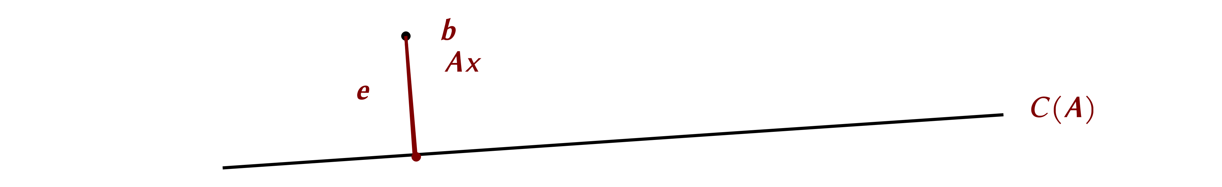
Given data 𝒃, form 𝑨, find 𝒙, such that || 𝒆 || = || 𝑨 𝒙 - 𝒃 || is minimized

𝒆 = 𝒃 - 𝑨 𝒙

The least-squares problem

focuses on a simpler representation of a data vector as a linear combination of column vectors of . Consider some phenomenon modeled as a function between vector spaces , such that for input parameters , the state of the system is . For most models is differentiable, a transcription of the condition that the system should not exhibit jumps in behavior when changing the input parameters. Then by appropriate choice of units and origin, a linearized model

𝒚 = 𝑨 𝒙, 𝑨 \in ℝ^{m \times n},

is obtained if , expressed as (1) if .

A simpler description is often sought, typically based on recognition that the inputs and outputs of the model can themselves be obtained as linear combinations , , involving a smaller set of parameters , , , . The column spaces of the matrices , are vector subspaces of the original set of inputs and outputs, , . The sets of column vectors of each form a reduced basis for the system inputs and outputs if they are chosed to be of full rank. The reduced bases are assumed to have been orthonormalized through the Gram-Schmidt procedure such that , and . Expressing the model inputs and outputs in terms of the reduced basis leads to

𝑪 𝒗 = 𝑨 𝑩 𝒖 \Rightarrow 𝒗 = 𝑪^{T} 𝑨 𝑩 𝒖 \Rightarrow 𝒗 = 𝑹 𝒖 .

The matrix is called the reduced system matrix and is associated with a mapping , that is a restriction to the vector subspaces of the mapping . When is an endomorphism, , , the same reduced basis is used for both inputs and outputs, , , and the reduced system is

𝒗 = 𝑹 𝒖, 𝑹 = 𝑩^{T} 𝑨 𝑩 .

Since is assumed to be orthogonal, the projector onto is . Applying the projector on the inital model

𝑷_{𝑩} 𝒚 = 𝑷_{𝑩} 𝑨 𝒙

leads to , and since the relation is obtained, and conveniently grouped as

𝑩 𝒗 = 𝑩 (𝑩^{T} 𝑨 𝑩) 𝒖 \Rightarrow 𝑩 𝒗 = 𝑩 (𝑹 𝒖),

again leading to the reduced model . The above calculation highlights that the reduced model is a projection of the full model on .

An often encountered situation is the reduction of large-dimensional dynamical system

\dot{𝒙} = \frac{d 𝒙}{d t}, \ddot{𝒙} = \frac{d \dot{𝒙}}{d t},

a generalization to multiple degrees of freedom of the damped oscillator equation

m \ddot{x} + d \dot{x} + k x = f .

In (), are the time-depenent coordinates of the system, the forces acting on the system, and are the mass, drag, stiffness matrices, respectively.

When , a reduced description is sought by linear combination of basis vectors

𝒙 ≅ \tilde{𝒙} = 𝑩 𝒚 \Rightarrow 𝑴 𝑩 \ddot{𝒚} + 𝑫 𝑩 \dot{𝒚} + 𝑲 𝑩 𝒚 = 𝒇

Choose to have orthonormal columns, and project () onto by multiplication with the projector

𝑩 𝑩^{T} 𝑴 𝑩 \ddot{𝒚} + 𝑩 𝑩^{T} 𝑫 𝑩 \dot{𝒚} + 𝑩 𝑩^{T} 𝑲 𝑩 𝒚 = 𝑩 𝑩^{T} 𝒇 \Rightarrow

𝑩 (𝑩^{T} 𝑴 𝑩 \ddot{𝒚} + 𝑩^{T} 𝑫 𝑩 \dot{𝒚} + 𝑩^{T} 𝑲 𝑩 𝒚 - 𝑩^{T} 𝒇) = 𝟎 \Leftrightarrow 𝑩 𝒛 = 𝟎 .

Since , deduce , hence

𝑩^{T} 𝑴 𝑩 \ddot{𝒚} + 𝑩^{T} 𝑫 𝑩 \dot{𝒚} + 𝑩^{T} 𝑲 𝑩 𝒚 = 𝑩^{T} 𝒇 .

Introduce notations

\tilde{𝑴} = 𝑩^{T} 𝑴 𝑩, \tilde{𝑫} = 𝑩^{T} 𝑫 𝑩, \tilde{𝑲} = 𝑩^{T} 𝑲 𝑩

for the reduced mass, drag, stiffness matrices, with , of smaller size. The reduced coordinates and forces are

\tilde{𝒇} = 𝑩^{T} 𝒇, 𝒚, \tilde{𝒇} \in ℝ^{n} .

The resulting reduced dynamical system is

\tilde{𝑴} \ddot{𝒚} + \tilde{𝑫} \dot{𝒚} + \tilde{𝑲} 𝒚 = \tilde{𝒇} .

One elemenet is missing from the description of model reduction above: how is determined? Domain-specific knowledge can often dictate an appropriate basis (e.g., Fourier basis fo periodic phenomena). An alternative approach is to extract an appropriate basis from observations of a phenomenon, known as data-driven modeling.

Consider two functions , that represent data streams in time of inputs and outputs of some system. A basic question arising in modeling and data science is whether the inputs and outputs are themselves in a functional relationship. This usually is a consequence of incomplete knowledge of the system, such that while might be assumed to be the most relevant input, output quantities, this is not yet fully established. A typical approach is to then carry out repeated measurements leading to a data set , thus defining a relation. Let denote vectors containing the input and output values. The mean values of the input and output are estimated by the statistics

μ_{1} ≅ {\overline{x}}_{1} = \frac{1}{N} \sum_{i = 1}^{N} x_{1} (t_{i}) = E [x_{1}], μ_{2} ≅ {\overline{x}}_{2} = \frac{1}{N} \sum_{i = 1}^{N} x_{2} (t_{i}) = E [x_{2}],

where is the expectation seen to be a linear mapping, whose associated matrix is

𝑬 = \frac{1}{N} [\begin{array}{llll} 1 & 1 & \dots & 1 \end{array}],

and the means are also obtained by matrix vector multiplication (linear combination),

{\overline{x}}_{1} = 𝑬 𝒙_{1}, {\overline{x}}_{2} = 𝑬 𝒙_{2} .

Deviation from the mean is measured by the standard deviation defined for by

σ_{1} = \sqrt{E [{(x_{1} - μ_{1})}^{2}]}, σ_{2} = \sqrt{E [{(x_{2} - μ_{2})}^{2}]} .

Note that the standard deviations are no longer linear mappings of the data.

Assume that the origin is chosen such that . One tool to estalish whether the relation is also a function is to compute the correlation coefficient

ρ (x_{1}, x_{2}) = \frac{E [x_{1} x_{2}]}{σ_{1} σ_{2}} = \frac{E [x_{1} x_{2}]}{\sqrt{E [x_{1}^{2}] E [x_{2}^{2}]}},

that can be expressed in terms of a scalar product and 2-norm as

ρ (x_{1}, x_{2}) = \frac{𝒙_{1}^{T} 𝒙_{2}}{{|| 𝒙_{1} ||}_{} {|| 𝒙_{2} ||}_{}} .

Squaring each side of the norm property , leads to

{(𝒙_{1} + 𝒙_{2})}^{T} (𝒙_{1} + 𝒙_{2}) ⩽ 𝒙_{1}^{T} 𝒙_{1} + 𝒙_{2}^{T} 𝒙_{2} + 2 || 𝒙_{1} || || 𝒙_{2} || \Rightarrow 𝒙_{1}^{T} 𝒙_{2} ⩽ || 𝒙_{1} || || 𝒙_{2} ||,

known as the Cauchy-Schwarz inequality, which implies . Depending on the value of , the variables are said to be:

uncorrelated, if ;
correlated, if ;
anti-correlated, if .

The numerator of the correlation coefficient is known as the covariance of

cov (x_{1}, x_{2}) = E [x_{1} x_{2}] .

The correlation coefficient can be interpreted as a normalization of the covariance, and the relation

cov (x_{1}, x_{2}) = 𝒙_{1}^{T} 𝒙_{2} = ρ (x_{1}, x_{2}) || 𝒙_{1} || || 𝒙_{2} ||,

is the two-variable version of a more general relationship encountered when the system inputs and outputs become vectors.

Consider now a related problem, whether the input and output parameters , thought to characterize a system are actually well chosen, or whether they are redundant in the sense that a more insightful description is furnished by with fewer components . Applying the same ideas as in the correlation coefficient, a sequence of measurements is made leading to data sets

𝑿 = [\begin{array}{llll} 𝒙_{1} & 𝒙_{2} & \dots & 𝒙_{n} \end{array}] \in ℝ^{N \times n}, 𝒀 = [\begin{array}{llll} 𝒚_{1} & 𝒚_{2} & \dots & 𝒚_{n} \end{array}] \in ℝ^{N \times m} .

Again, by appropriate choice of the origin the means of the above measurements is assumed to be zero

E [𝒙] = 𝟎, E [𝒚] = 𝟎 .

Covariance matrices can be constructed by

𝑪_{𝑿} = 𝑿^{T} 𝑿 = [\begin{array}{l} 𝒙_{1}^{T} \\ 𝒙_{2}^{T} \\ ⋮ \\ 𝒙_{n}^{T} \end{array}] [\begin{array}{llll} 𝒙_{1} & 𝒙_{2} & \dots & 𝒙_{n} \end{array}] = [\begin{array}{llll} 𝒙_{1}^{T} 𝒙_{1} & 𝒙_{1}^{T} 𝒙_{2} & \dots & 𝒙_{1}^{T} 𝒙_{n} \\ 𝒙_{2}^{T} 𝒙_{1} & 𝒙_{2}^{T} 𝒙_{2} & \dots & 𝒙_{2}^{T} 𝒙_{n} \\ ⋮ & ⋮ & ⋱ & ⋮ \\ 𝒙_{n}^{T} 𝒙_{1} & 𝒙_{n}^{T} 𝒙_{2} & \dots & 𝒙_{n}^{T} 𝒙_{n} \end{array}] \in ℝ^{n \times n} .

Consider now the SVDs of , , and from

𝑪_{𝑿} = 𝑿^{T} 𝑿 = {(𝑼 𝚺 𝑺^{T})}^{T} 𝑼 𝚺 𝑺^{T} = 𝑺 𝚺^{T} 𝑼^{T} 𝑼 𝚺 𝑺^{T} = 𝑺 𝚺^{T} 𝚺 𝑺^{T} = 𝑵 𝚲 𝑵^{T},

identify , and .

Recall that the SVD returns an order set of singular values , and associated singular vectors. In many applications the singular values decrease quickly, often exponentially fast. Taking the first singular modes then gives a basis set suitable for mode reduction

𝒙 = 𝑺_{q} 𝒖 = [\begin{array}{llll} 𝒔_{1} & 𝒔_{2} & \dots & 𝒔_{q} \end{array}] 𝒖 .

The data reduction inherent in SVD representations is a generic feature of natural phenomena. A paradigm for physical systems is the evolution of correlated behavior against a backdrop of thermal enery, typically represented as a form of noise.

One mathematical technique to model such systems is the definition of a stochastic process , where for each fixed , is a random variable, i.e., a measurable function from a set of possible outcomes to a measurable space . The set is the sample space of a probability triple , where for

P (X \in S) = P ({ω \in Ω} | X (ω) \in S |) .

A measurable space is a set coupled with procedure to determine measurable subsets, known as a -algebra.

Suppose now that admits a unique solution with , , known as a square system of linear equations where the number of unknowns equals that of the equations. How to find it? We are especially interested in constructing a general procedure, that will work no matter what the size of might be. This means we seek an algorithm that precisely specifies the steps that lead to the solution, and that we can program a computing device to carry out automatically. One such algorithm is Gaussian elimination.

Consider the system

{\begin{array}{ccc} x_{1} + 2 x_{2} - x_{3} & = & 2 \\ 2 x_{1} - x_{2} + x_{3} & = & 2 \\ 3 x_{1} - x_{2} - x_{3} & = & 1 \end{array} .

The idea is to combine equations such that we have one fewer unknown in each equation. Ask: with what number should the first equation be multiplied in order to eliminate from sum of equation 1 and equation 2? This number is called a Gaussian multiplier, and is in this case . Repeat the question for eliminating from third equation, with multiplier .

{\begin{array}{ccc} x_{1} + 2 x_{2} - x_{3} & = & 2 \\ 2 x_{1} - x_{2} + x_{3} & = & 2 \\ 3 x_{1} - x_{2} - x_{3} & = & 1 \end{array} . \Rightarrow {\begin{array}{ccc} x_{1} + 2 x_{2} - x_{3} & = & 2 \\ - 5 x_{2} + 3 x_{3} & = & - 2 \\ - 7 x_{2} + 2 x_{3} & = & - 5 \end{array} .

Now, ask: with what number should the second equation be multiplied to eliminate from sum of second and third equations. The multiplier is in this case .

{\begin{array}{ccc} x_{1} + 2 x_{2} - x_{3} & = & 2 \\ - 5 x_{2} + 3 x_{3} & = & - 2 \\ - 7 x_{2} + 2 x_{3} & = & - 5 \end{array} . \Rightarrow {\begin{array}{ccc} x_{1} + 2 x_{2} - x_{3} & = & 2 \\ - 5 x_{2} + 3 x_{3} & = & - 2 \\ - \frac{11}{5} x_{3} & = & - \frac{11}{5} \end{array} .

Starting from the last equation we can now find , replace in the second to obtain , hence , and finally replace in the first equation to obtain .

The above operations only involve coefficients. A more compact notation is therefore to work with what is known as the "bordered matrix"

(\begin{array}{cccc} 1 & 2 & - 1 & 2 \\ 2 & - 1 & 1 & 2 \\ 3 & - 1 & - 1 & 1 \end{array}) \sim (\begin{array}{cccc} 1 & 2 & - 1 & 2 \\ 0 & - 5 & 3 & - 2 \\ 0 & - 7 & 2 & - 5 \end{array}) \sim (\begin{array}{cccc} 1 & 2 & - 1 & 2 \\ 0 & - 5 & 3 & - 2 \\ 0 & 0 & - \frac{11}{5} & - \frac{11}{5} \end{array})

Once the above triangular form has been obtain, the solution is found by back substitution, in which we seek to form the identity matrix in the first 3 columns, and the solution is obtained in the last column.

(\begin{array}{cccc} 1 & 2 & - 1 & 2 \\ 0 & - 5 & 3 & - 2 \\ 0 & 0 & - \frac{11}{5} & - \frac{11}{5} \end{array}) \sim (\begin{array}{cccc} 1 & 2 & - 1 & 2 \\ 0 & - 5 & 3 & - 2 \\ 0 & 0 & 1 & 1 \end{array}) \sim (\begin{array}{cccc} 1 & 0 & 0 & 1 \\ 0 & 1 & 0 & 1 \\ 0 & 0 & 1 & 1 \end{array})

We have introduced Gaussian elimination as a procedure to solve the linear system ("find coordinates of vector in terms of column vectors of matrix "),
We now reinterpret Gaussian elimination as a sequence of matrix multiplications applied to to obtain a simpler, upper triangular form.

Consider the system

{\begin{array}{ccc} x_{1} + 2 x_{2} - x_{3} & = & 2 \\ 2 x_{1} - x_{2} + x_{3} & = & 2 \\ 3 x_{1} - x_{2} - x_{3} & = & 1 \end{array} .

with

A = (\begin{array}{ccc} 1 & 2 & - 1 \\ 2 & - 1 & 1 \\ 3 & - 1 & - 1 \end{array}), b = (\begin{array}{c} 2 \\ 2 \\ 1 \end{array})

We ask if there is a matrix that could be multiplied with to produce a result with zeros under the main diagonal in the first column. First, gain insight by considering multiplication by the identity matrix, which leaves unchanged

(\begin{array}{ccc} 1 & 0 & 0 \\ 0 & 1 & 0 \\ 0 & 0 & 1 \end{array}) (\begin{array}{ccc} 1 & 2 & - 1 \\ 2 & - 1 & 1 \\ 3 & - 1 & - 1 \end{array}) = (\begin{array}{ccc} 1 & 2 & - 1 \\ 2 & - 1 & 1 \\ 3 & - 1 & - 1 \end{array})

In the first stage of Gaussian multiplication, the first line remains unchanged, so we deduce that should have the same first line as the identity matrix

L_{1} = (\begin{array}{ccc} 1 & 0 & 0 \\ ? & ? & ? \\ ? & ? & ? \end{array})

(\begin{array}{ccc} 1 & 0 & 0 \\ ? & ? & ? \\ ? & ? & ? \end{array}) (\begin{array}{ccc} 1 & 2 & - 1 \\ 2 & - 1 & 1 \\ 3 & - 1 & - 1 \end{array}) = (\begin{array}{ccc} 1 & 2 & - 1 \\ 0 & - 5 & 3 \\ 0 & - 7 & 2 \end{array})

Next, recall the way Gaussian multipliers were determined: find number to multiply first line so that added to second, third lines a zero is obtained. This leads to the form

L_{1} = (\begin{array}{ccc} 1 & 0 & 0 \\ ? & 1 & 0 \\ ? & 0 & 1 \end{array})

Finally, identify the missing entries with the Gaussian multipliers to determine

L_{1} = (\begin{array}{ccc} 1 & 0 & 0 \\ - 2 & 1 & 0 \\ - 3 & 0 & 1 \end{array})

Verify by carrying out the matrix multiplication

L_{1} A = (\begin{array}{ccc} 1 & 0 & 0 \\ - 2 & 1 & 0 \\ - 3 & 0 & 1 \end{array}) (\begin{array}{ccc} 1 & 2 & - 1 \\ 2 & - 1 & 1 \\ 3 & - 1 & - 1 \end{array}) = (\begin{array}{ccc} 1 & 2 & - 1 \\ 0 & - 5 & 3 \\ 0 & - 7 & 2 \end{array})

Repeat the above reasoning to come up with a second matrix that forms a zero under the main diagonal in the second column

L_{2} = (\begin{array}{ccc} 1 & 0 & 0 \\ 0 & 1 & 0 \\ 0 & - 7 / 5 & 1 \end{array})

L_{2} L_{1} A = (\begin{array}{ccc} 1 & 0 & 0 \\ 0 & 1 & 0 \\ 0 & - 7 / 5 & 1 \end{array}) (\begin{array}{ccc} 1 & 2 & - 1 \\ 0 & - 5 & 3 \\ 0 & - 7 & 2 \end{array}) = (\begin{array}{ccc} 1 & 2 & - 1 \\ 0 & - 5 & 3 \\ 0 & 0 & - 11 / 5 \end{array}) = U

We have obtained a matrix with zero entries under the main diagonal (an upper triangular matrix) by a sequence of matrix multiplications.

From the above, we assume that we can form a sequence of multiplier matrices such that the result is an upper triangular matrix

L_{m - 1} . . . L_{2} L_{1} A = U

Recall the basic operation in row echelon reduction: constructing a linear combination of rows to form zeros beneath the main diagonal, e.g.
$𝑨 = \sim$
This can be stated as a matrix multiplication operation, with
$=$

For nonsingular, the successive steps in row echelon reduction (or Gaussian elimination) correspond to successive multiplications on the left by Gaussian multiplier matrices
$𝑳_{m - 1} 𝑳_{m - 2} \dots 𝑳_{2} 𝑳_{1} 𝑨 = 𝑼$
The inverse of a Gaussian multiplier is
$𝑳_{k}^{- 1} = = 𝑰 - (𝑳_{k} - 𝑰)$

From obtain
$𝑨 = {(𝑳_{m - 1} 𝑳_{m - 2} \dots 𝑳_{2} 𝑳_{1})}^{- 1} 𝑼 = 𝑳_{1}^{- 1} 𝑳_{2}^{- 1} \cdot \dots \cdot 𝑳_{m - 1}^{- 1} 𝑼 = 𝑳 𝑼$
Due to the simple form of the matrix is easily obtained as
$𝑳 =$

We will show that this indeed possible if admits a unique solution. Furthermore, the product of lower triangular matrices is lower triangular, and the inverse of a lower triangular matrix is lower triangular (same applies for upper triangular matrices). Introduce the notation

L^{- 1} = L_{m - 1} . . . L_{2} L_{1}

and obtain

L^{- 1} A = U

A = L U

The above result permits a basic insight into Gaussian elimination: the procedure depends on "factoring" the matrix into two "simpler" matrices . The idea of representing a matrix as a product of simpler matrices is fundamental to linear algebra, and we will come across it repeatedly.

For now, the factorization allows us to devise the following general approach to solving

Find the factorization
Insert the factorization into to obtain , where the notation has been introduced. The system
$L y = b$
is easy to solve by forward substitution to find for given
Finally find by backward substitution solution of
$U x = y$

Given

By analogy to the simple scalar equation with solution when , we are interested in writing the solution to a linear system as for , . Recall that solving corresponds to expressing the vector as a linear combination of the columns of . This can only be done if the columns of form a basis for , in which case we say that is non-singular.

Computation of the inverse can be carried out by repeated use of Gauss elimination. Denote the inverse by for a moment and consider the inverse matrix property . Introducing the column notation for leads to

A (\begin{array}{ccc} B_{1} & . . . & B_{m} \end{array}) = (\begin{array}{ccc} e_{1} & . . . & e_{m} \end{array})

and identification of each column in the equality states

A B_{k} = e_{k}, k = 1, 2, . ., m

with the column unit vector with zero components everywhere except for a in row . To find the inverse we need to simultaneously solve the linear systems given above.

Gauss-Jordan algorithm example. Consider

A = (\begin{array}{ccc} 1 & 2 & 3 \\ - 1 & 3 & 1 \\ 2 & - 1 & - 2 \end{array})

To find the inverse we solve the systems . This can be done simultaneously by working with the matrix bordered by

(A | I) = (\begin{array}{cccccc} 1 & 1 & 0 & 1 & 0 & 0 \\ - 1 & 1 & 1 & 0 & 1 & 0 \\ 2 & 4 & - 2 & 0 & 0 & 1 \end{array})

Carry out now operations involving linear row combinations and permutations to bring the left side to

(\begin{array}{cccccc} 1 & 1 & 0 & 1 & 0 & 0 \\ - 1 & 1 & 1 & 0 & 1 & 0 \\ 2 & 4 & - 2 & 0 & 0 & 1 \end{array}) \sim (\begin{array}{cccccc} 1 & 1 & 0 & 1 & 0 & 0 \\ 0 & 2 & 1 & 1 & 1 & 0 \\ 0 & 2 & - 2 & - 2 & 0 & 1 \end{array}) \sim (\begin{array}{cccccc} 1 & 1 & 0 & 1 & 0 & 0 \\ 0 & 2 & 1 & 1 & 1 & 0 \\ 0 & 0 & - 3 & - 3 & - 1 & 1 \end{array}) \sim

\sim (\begin{array}{cccccc} 1 & 1 & 0 & 1 & 0 & 0 \\ 0 & 2 & 1 & 1 & 1 & 0 \\ 0 & 0 & 1 & 1 & \frac{1}{3} & - \frac{1}{3} \end{array}) \sim (\begin{array}{cccccc} 1 & 1 & 0 & 1 & 0 & 0 \\ 0 & 2 & 0 & 0 & \frac{2}{3} & \frac{1}{3} \\ 0 & 0 & 1 & 1 & \frac{1}{3} & - \frac{1}{3} \end{array}) \sim (\begin{array}{cccccc} 1 & 1 & 0 & 1 & 0 & 0 \\ 0 & 1 & 0 & 0 & \frac{1}{3} & \frac{1}{6} \\ 0 & 0 & 1 & 1 & \frac{1}{3} & - \frac{1}{3} \end{array}) \sim

(\begin{array}{cccccc} 1 & 0 & 0 & 1 & - \frac{1}{3} & - \frac{1}{6} \\ 0 & 1 & 0 & 0 & \frac{1}{3} & \frac{1}{6} \\ 0 & 0 & 1 & 1 & \frac{1}{3} & - \frac{1}{3} \end{array})

to obtain

A^{- 1} = (\begin{array}{ccc} 1 & - \frac{1}{3} & - \frac{1}{6} \\ 0 & \frac{1}{3} & \frac{1}{6} \\ 1 & \frac{1}{3} & - \frac{1}{3} \end{array})

The basic procedures within factorization can be adapted to account for special structure of the system matrix or to obtain properties associated with .

a square matrix, is the oriented volume enclosed by the column vectors of (a parallelipiped)
Geometric interpretation of determinants
Determinant calculation rules
Algebraic definition of a determinant

$𝑨 =,, \det (𝑨) =$
$𝑨 =,, \det (𝑨) =$

Computation of a determinant with
$= a_{11} a_{22} - a_{12} a_{21}$
Computation of a determinant with
Where do these determinant computation rules come from? Two viewpoints
- Geometric viewpoint: determinants express parallelepiped volumes
- Algebraic viewpoint: determinants are computed from all possible products that can be formed from choosing a factor from each row and each column

In two dimensions a “parallelepiped” becomes a parallelogram with area given as
$(Area) = (Length of Base) \times (Length of Height)$
Take as the base, with length . Vector is at angle to -axis, is at angle to -axis, and the angle between , is . The height has length
$h = || 𝒂_{2} || \sin θ = || 𝒂_{2} || \sin . (. φ_{2} - φ_{1}) = || 𝒂_{2} || (\sin φ_{2} \cos φ_{1} - \sin φ_{1} \cos φ_{2})$
Use , , ,
$(Area) = || 𝒂_{1} || || 𝒂_{2} || (\sin φ_{2} \cos φ_{1} - \sin φ_{1} \cos φ_{2}) = a_{11} a_{22} - a_{12} a_{21}$

The geometric interpretation of a determinant as an oriented volume is useful in establishing rules for calculation with determinants:
- Determinant of matrix with repeated columns is zero (since two edges of the parallelepiped are identical). Example for
  $Δ = = a b w + b c u + c a v - u b c - v c a - w a b = 0$
  This is more easily seen using the column notation
  $Δ = \det = 0$
- Determinant of matrix with linearly dependent columns is zero (since one edge lies in the 'hyperplane' formed by all the others)

Separating sums in a column (similar for rows)
$\det = \det + \det$
with
Scalar product in a column (similar for rows)
$\det = α \det$
with
Linear combinations of columns (similar for rows)
$\det = \det$
with .

A determinant of size can be expressed as a sum of determinants of size by expansion along a row or column

The formal definition of a determinant
$\det A = \sum_{σ \in Σ} ν (σ) a_{1 i_{1}} a_{2 i_{2}} \dots a_{m i_{m}}$
requires operations, a number that rapidly increases with
A more economical determinant is to use row and column combinations to create zeros and then reduce the size of the determinant, an algorithm reminiscent of Gauss elimination for systems

Example:
$= = = 20 - 12 = 8$
The first equality comes from linear combinations of rows, i.e. row 1 is added to row 2, and row 1 multiplied by 2 is added to row 3. These linear combinations maintain the value of the determinant. The second equality comes from expansion along the first column

Consider . We've introduced the idea of a scalar product
$u \cdot v = u^{T} v = u_{1} v_{1} + u_{2} v_{2} + u_{3} v_{3}$
in which from two vectors one obtains a scalar
We've also introduced the idea of an exterior product
$u v^{T} = =$
in which a matrix is obtained from two vectors
Another product of two vectors is also useful, the cross product, most conveniently expressed in determinant-like form
$u \times v = = (u_{2} v_{3} - v_{2} u_{3}) 𝒆_{1} + (u_{3} v_{1} - v_{3} u_{1}) 𝒆_{2} + (u_{1} v_{2} - v_{1} u_{2}) 𝒆_{3}$

The special structure of a matrix can be exploited to obtain more efficient factorizations. Evaluation of the linear combination requires floating point operations (flops) for . Evaluation of linear combinations , requires flops. If it is possible to evaluate with fewer operations, the matrix is said to be structured. Examples include:

Banded matrices , if or , with denoting the lower and upper bandwidths. If the matrix is diagonal. If the matrix is said to have bandwidth , i.e., for , the matrix is tridiagonal, and for the matrix is pentadiagonal. Lower triangular matrices have , while upper triangular matrices have . The product requires flops.
Sparse matrices have non-zero elements per row or non-zero elements per column. The product requires or flops
Circulant matrices are sqaure and have , a property that can be exploited to compute using operations
For square, rank-deficient matrices , , can be evaluated in flops
When are symmetric (hence square), requires flops instead of .

Special structure of a matrix is typically associated with underlying symmetries of a particular phenomenon. For example, the law of action and reaction in dynamics (Newton's third law) leads to real symmetric matrices, , . Consider a system of point masses with nearest-neighbor interactions on the real line where the interaction force depends on relative position. Assume that the force exerted by particle on particle is linear

f_{i + 1, i} = f (u_{i + 1} - u_{i}) = k (u_{i + 1} - u_{i}),

with denoting displacement from an equilibrium position. The law of action and reaction then states that

f_{i, i + 1} = - f_{i + 1, i} = k (u_{i} - u_{i + 1}) .

If the same force law holds at all positions, then

f_{i - 1, i} = k (u_{i - 1} - u_{i}) .

The force on particle is given by the sum of forces from neighboring particles

f_{i} = f_{i - 1, i} + f_{i + 1, i} = k (u_{i - 1} - u_{i}) + k (u_{i + 1} - u_{i}) = k (u_{i + 1} - 2 u_{i} + u_{i - 1}) .

Introducing , and assuming , the above is stated as

𝒇 = 𝑲 𝒖,

with is a symmetric matrix, , a direct consequence of the law of action and reaction. The matrix is in this case tridiagonal as a consequence of the assumption of nearest-neighbor interactions. Recall that matrices represent linear mappings, hence

𝑲 = [\begin{array}{llll} 𝒇 (𝒆_{1}) & 𝒇 (𝒆_{2}) & \dots & 𝒇 (𝒆_{m}) \end{array}],

with the force-displacement linear mapping, Fig. , obtaining the same symmetric, tri-diagonal matrix.

This concept can be extended to complex matrices through , in which case is said to be self-adjoint or hermitian. Again, this property is often associated with desired physical properties, such as the requirement of real observable quantitites in quantum mechanics. Diagonal elements of a hermitian matrix must be real, and for any , the computation

\overline{𝒙^{*} 𝑨 𝒚} = {(𝒙^{*} 𝑨 𝒚)}^{*} = 𝒚^{*} 𝑨^{*} 𝒙 = 𝒚^{*} 𝑨^{} 𝒙,

implies for that

\overline{𝒙^{*} 𝑨 𝒙} = 𝒙^{*} 𝑨 𝒙,

hence is real.

The work (i.e., energy stored in the system) done by all the forces in the above point mass system is

𝒲 = \frac{1}{2} 𝒖^{T} 𝑲 𝒖,

and physical considerations state that . This leads the following definitions.

If is hermitian positive definite, then so is for any . Choosing

𝑿 = [\begin{array}{lll} 𝒆_{1} & \dots & 𝒆_{n} \end{array}] \in ℂ^{m \times n}

gives , the principal submatrix of , itself a hermitian positive definite matrix. Choosing shows that the diagonal element of is positive,

The structure of a hermitian positive definite matrix , can be preserved by modification of -factorization. The resulting algorithm is known as Cholesky factorization, and its first stage is stated as

𝑨 = [\begin{array}{ll} a_{11} & 𝒘^{*} \\ 𝒘 & 𝑩 \end{array}] = [\begin{array}{ll} α & 𝟎 \\ 𝒘 / α & 𝑰 \end{array}] [\begin{array}{ll} 1 & 𝟎^{*} \\ 𝟎 & 𝑪 \end{array}] [\begin{array}{ll} α & 𝒘^{*} / α \\ 𝟎 & 𝑰 \end{array}] = [\begin{array}{ll} α & 𝟎 \\ 𝒘 / α & 𝑰 \end{array}] [\begin{array}{ll} α & 𝒘^{*} / α \\ 𝟎 & 𝑪 \end{array}] = [\begin{array}{ll} a_{11} & 𝒘^{*} \\ 𝒘 & 𝑪 + 𝒘 𝒘^{*} / a_{11} \end{array}],

whence . Repeating the stage-1 step

𝑨 = 𝑳_{1} 𝑨_{1} 𝑳_{1}^{*},

leads to

𝑨 = 𝑳_{1} 𝑳_{2} 𝑨_{2} 𝑳_{2}^{*} 𝑳_{1}^{*} = \dots = 𝑳 𝑳^{*}, 𝑳 = 𝑳_{1} 𝑳_{2} \dots 𝑳_{m} .

The resulting Cholesky algorithm is half as expensive as standard -factorization.

Linear endomorphisms , represented by , can exhibit invariant directions for which

𝒇 (𝒙) = 𝑨 𝒙 = λ 𝒙,

known as eigenvectors, with associated eigenvalue . Eigenvectors are non-zero elements of the null space of ,

(𝑨 - λ 𝑰) 𝒙 = 𝟎,

and the null-space is referred to as the eigenspace of for eigenvalue , .

Non-zero solutions are obtained if is rank-deficient (singular), or has linearly dependent columns in which case

\det (𝑨 - λ 𝑰) = 0 \Rightarrow \det (λ 𝑰 - 𝑨) = = 0 .

From the determinant definition as “sum of all products choosing an element from row/column”, it results that

\det (λ 𝑰 - 𝑨) = λ^{m} + c_{1} λ^{m - 1} + \dots + c_{m - 1} λ + c_{m} = p_{A} (λ),

known as the characteristic polynomial associated with the matrix 𝑨, and of degree . The characteristic polynomial is monic, meaning that the coefficient of the highest power is equal to one. The fundamental theorem of algebra states that of degree has roots, hence has eigenvalues (not necessarily distinct), and associated eigenvectors. This can be stated in matrix form as

𝑨 𝑿 = 𝑿 𝚲,

with

𝑿 = [\begin{array}{lll} 𝒙_{1} & \dots & 𝒙_{m} \end{array}], 𝚲 = diag (λ_{1}, \dots, λ_{m}),

the eigenvector matrix and eigenvalue matrix, respectively. By definition, the matrix is diagonalizable if is of full rank, in which case the eigendecomposition of is

𝑨 = 𝑿 𝚲 𝑿^{- 1} .

The statement , that eigenvector is an invariant direction of the operator along which the effect of operator is scaling by , suggests that similar behavior would be obtained under a coordinate transformation . Assuming is of full rank and introducing , this leads to

𝑨 𝒙 = 𝑨 𝑻 𝒚 = λ 𝒙 = λ 𝑻 𝒚 \Rightarrow 𝑻^{- 1} 𝑨 𝑻 𝒚 = λ 𝒚 .

Upon coordinate transformation, the eigenvalues (scaling factors along the invariant directions) stay the same. Metric-preserving coordinate transformations are of particular interest, in which case the transformation matrix is unitary .

Since the eigenvalues of are the same, and a polynomial is completely specified by its roots and coefficient of highest power, the characteristic polynomials of must be the same

p_{𝑨} (λ) = \prod_{k = 1}^{m} (λ - λ_{k}) = p_{𝑩} (λ) .

This can also be verified through the determinant definition

p_{𝑩} (t) = \det (λ 𝑰 - 𝑩) = \det (λ 𝑻^{- 1} 𝑻 - 𝑻^{- 1} 𝑨 𝑻) = \det (𝑻^{- 1} (λ 𝑰 - 𝑨) 𝑻) = \det (𝑻^{- 1}) \det (λ 𝑰 - 𝑨) \det (𝑻) = p_{𝑨} (λ),

since .

A solution to the eigenvalue problem always exists, but the eigenvectors of do not always form a basis set, i.e., is not always of full rank. The factorized form of the characteristic polynomial of is

p_{𝑨} (λ) = \det (λ 𝑰 - 𝑨) = \prod_{k = 1}^{K} {(λ - λ_{k})}_{}^{m_{k}},

with denoting the number of distinct roots of , and is the algebraic multiplicity of eigenvalue , defined as the number of times the root is repeated. Let denote the associated eigenspace . The dimension of denoted by is the geometric multiplicity of eigenvalue . The eigenvector matrix is of full rank when the vector sum of the eigenspaces covers , as established by the following results.

Eigenvalues as roots of the characteristic polynomial

p_{A} (λ) = \det (λ 𝑰 - 𝑨) = λ^{m} + c_{1} λ^{m - 1} + \dots + c_{m - 1} λ + c_{m} = \prod_{k = 1}^{m} (λ - λ_{k})

reveal properties of a matrix . The evaluation of leads to

\det (- 𝑨) = {(- 1)}^{m} \det (𝑨) = {(- 1)}^{m} \prod_{k = 1}^{m} λ_{k},

hence the determinant of a matrix is given by the product of its eigenvalues

\det (𝑨) = \prod_{k = 1}^{m} λ_{k} .

The trace of a matrix is the sum of its diagonal elements is equal to the sum of its eigenvalues

tr (𝑨) = \sum_{k = 1}^{m} a_{k k} = \sum_{k = 1}^{m} λ_{k},

a relationship established by the Vieta formulas.

Whereas the SVD, QR, LU decompositions can be applied to general matrices with not necessarily equal to , the eigendecomposition requires , and hence is especially relevant in the characterization of endomorphisms. A generic time evolution problem is stated as

\partial_{t} 𝒖 = 𝒖_{t} = 𝒇 (𝒖), 𝒖 (0) = 𝒖_{0}, 𝒖 : ℝ_{+} \to ℂ^{m},

stating that the rate of change in the state variables characterizing some system is a function of the current state through the function , an endomorphism. An approximation of is furnished by the MacLaurin series

𝒇 (𝒖) = 𝒗 + 𝑨 𝒖 + 𝒪 ({|| 𝒖 ||}^{2}), 𝒗 = 𝒇 (𝟎), 𝑨 = \frac{\partial 𝒇}{\partial 𝒖} (𝟎) .

Truncation at first order gives a linear ODE system , that can be formally integrated to give

𝒖 (t) = 𝒗 t + e^{t 𝑨} 𝒖_{0} .

The matrix exponential is defined as

e^{t 𝑨} = 𝑰 + \frac{1}{1!} t 𝑨 + \frac{1}{2!} {(t 𝑨)}^{2} + \frac{1}{3!} {(t 𝑨)}^{3} + \dots .

Evaluation of requires matrix multiplications or floating point operations. However, if the eigendecomposition of is available the matrix exponential can be evaluate in only operations since

𝑨^{k} = (𝑿 𝚲 𝑿^{- 1}) (𝑿 𝚲 𝑿^{- 1}) \dots (𝑿 𝚲 𝑿^{- 1}) = 𝑿 𝚲^{k} 𝑿^{- 1},

leads to

e^{t 𝑨} = 𝑿 e^{t 𝚲} 𝑿^{- 1} .

The existence of the SVD was establish by a constructive procedure by complete induction. However the proof depends on determining the singular values, e.g., . The existence of the singular values was established by an argument from analysis, that the norm function on a compact domain must attain its extrema. This however leaves open the problem of effectively determining the singular values. In practive the singular values and vectors are determined by solving the eigenvalue problem for and

𝑨^{*} 𝑨 = {(𝑼 𝚺 𝑽^{*})}^{*} (𝑼 𝚺 𝑽^{*}) = 𝑽 𝚺^{T} 𝑼^{*} 𝑼 𝚺 𝑽^{*} = 𝑽 𝚺^{T} 𝚺 𝑽^{*} \Rightarrow (𝑨^{*} 𝑨) 𝑽 = 𝑽 𝚺^{T} 𝚺,

𝑨 𝑨^{*} = (𝑼 𝚺 𝑽^{*}) {(𝑼 𝚺 𝑽^{*})}^{*} = 𝑼 𝚺 𝑽^{*} 𝑽 𝚺^{T} 𝑼^{*} = 𝑼 𝚺 𝚺^{T} 𝑼^{*} \Rightarrow (𝑨 𝑨^{*}) 𝑼 = 𝑼 𝚺 𝚺^{T} .

From the above the left singular vectors are eigenvectors of , and the right singular vectors are eigenvectors of . Both and have the same eigenvalues that are the squared singular values.

The relevance of eigendecompositions to repeated application of the linear operator as in

𝒆^{t 𝑨} = 𝑰 + \frac{1}{1!} t 𝑨 + \frac{1}{2!} t^{2} 𝑨^{2} + \dots = 𝑿 e^{t 𝚲} 𝑿^{- 1},

suggests that algorithms that construct powers of might reveal eigenvalues. This is indeed the case and leads to a class of algorithms of wide applicability in scientific computation. First, observe that taking condition numbers gives

μ (𝑨) = μ (𝑿 𝚲 𝑿^{- 1}) ⩽ μ^{2} (𝑿) μ (𝚲) = ({| λ |}_{max} / {| λ |}_{min}),

where , are the eigenvalues of maximum and minimum absolute values. While these express an intrinsic property of the operator , the factor is associated with the conditioning of a change of coordinates, and a natural question is whether it is possible to avoid any ill-conditioning associated with a basis set that is close to linear dependence. The answer to this line of inquiry is given by the following result.

The eigenvalues of an upper triangular matrix are simply its diagonal elements, so the Schur factorization is an eigenvalue-revealing factorization.

When the operator expresses some physical phenomenon, the principle of action and reaction implies that is symmetric, and has real eigenvalues. Componentwise, symmetry of implies . Consider , and take the adjoint to obtain , or since is symmetric. Form scalar products , , and subtract to obtain

0 = (λ - \overline{λ}) 𝒙^{T} 𝒙 \Rightarrow λ = \overline{λ} \Rightarrow λ \in ℝ,

since , an eigenvector.

For a real symmetric matrix the Schur theorem states that

𝑨 = 𝑨^{T} \Rightarrow (𝑸 𝑻 𝑸^{T}) = 𝑸 𝑻^{T} 𝑸^{T} \Rightarrow 𝑻 = 𝑻^{T},

and since a symmetric triangular matrix is diagonal, the Schur factorization is also an eigendecomposition, and the eigenvector matrix is a basis, .

Assume initially that the eigenvalues are distinct and ordered . Repeated application of on an arbitrary vector is expressed as

𝑨^{n} 𝒗 = {(𝑸 𝚲 𝑸^{T})}^{n} 𝑸 𝒄 = (𝑸 𝚲 𝑸^{T}) (𝑸 𝚲 𝑸^{T}) \dots (𝑸 𝚲 𝑸^{T}) 𝑸 𝒄 = 𝑸 𝚲^{n} 𝒄,

a linear combination of the columns of (eigenvectors of ) with coefficients .

The sequence of normalized eigenvector approximants is linearly convergent at rate .

To estimate the eigenvalue revealed by power iteration, formulate the least squares problem

{min}_{c} || 𝑨 𝒗 - 𝒗 c ||,

that seeks the best approximation of one power iteration as a linear combination of the initial vector . Of course, if is an eigenvector, then the solution would be , the associated eigenvalue. The projector onto is

𝑷 = \frac{𝒗 𝒗^{T}}{𝒗^{T} 𝒗},

that when applied to gives the equation

𝑷 𝑨 𝒗 = \frac{𝒗 𝒗^{T}}{𝒗^{T} 𝒗} 𝑨 𝒗 = \frac{𝒗^{T} 𝑨 𝒗}{𝒗^{T} 𝒗} 𝒗 = c 𝒗 \Rightarrow c = \frac{𝒗^{T} 𝑨 𝒗}{𝒗^{T} 𝒗} .

The function ,

r (𝒗) = \frac{𝒗^{T} 𝑨 𝒗}{𝒗^{T} 𝒗},

is known as the Rayleigh quotient which, evaluated for an eigenvector, gives . To determine how well the eigenvalue is approximated, carry out a Taylor series in the vicinity of an eigenvector

r (𝒗) = r (𝒒) + \frac{1}{1!} {[\nabla_{𝒗} r (𝒒)]}^{T} (𝒗 - 𝒒) + 𝒪 ({|| 𝒗 - 𝒒 ||}^{2}),

where is the gradient of

\nabla_{𝒗} r = [\begin{array}{l} \frac{\partial r}{\partial v_{1}} \\ ⋮ \\ \frac{\partial r}{\partial v_{m}} \end{array}] .

Compute the gradient through differentiation of the Rayleigh quotient

\nabla_{𝒗} r (𝒗) = \frac{\nabla_{𝒗} (𝒗^{T} 𝑨 𝒗)}{𝒗^{T} 𝒗} - \frac{(𝒗^{T} 𝑨 𝒗)}{{(𝒗^{T} 𝒗)}^{2}} \nabla_{𝒗} (𝒗^{T} 𝒗) .

Noting that , the column of , the gradient of is

\nabla_{𝒗} (𝒗^{T} 𝒗) = \nabla_{𝒗} \sum_{i = 1}^{m} v_{i}^{2} = \sum_{i = 1}^{m} \nabla_{𝒗} v_{i}^{2} = \sum_{i = 1}^{m} 2 v_{i} \nabla_{𝒗} v_{i} = 2 \sum_{i = 1}^{m} v_{i} 𝒆_{i} = 2 𝒗 .

To compute , let , and since is symmetric , leading to

\nabla_{𝒗} (𝒗^{T} 𝑨 𝒗) = \nabla_{𝒗} (𝒖^{T} 𝒗) = \sum_{i = 1}^{m} \nabla_{𝒗} (u_{i} v_{i}) = \sum_{i = 1}^{m} u_{i} \nabla_{𝒗} v_{i} + \sum_{i = 1}^{m} v_{i} \nabla_{𝒗} u_{i} .

Use also expressed as by swapping indices to obtain

\nabla_{𝒗} u_{i} = \sum_{j = 1}^{m} a_{i j} \nabla_{𝒗} v_{j} = \sum_{j = 1}^{m} a_{i j} 𝒆_{j}

and therefore

\sum_{i = 1}^{m} v_{i} \nabla_{𝒗} u_{i} = \sum_{i = 1}^{m} v_{i} \sum_{j = 1}^{m} a_{i j} 𝒆_{j} = \sum_{j = 1}^{m} \sum_{i = 1}^{m} a_{i j} v_{i} 𝒆_{j} = \sum_{j = 1}^{m} \sum_{i = 1}^{m} a_{i j} v_{i} 𝒆_{j} .

Use symmetry of to write

\sum_{i = 1}^{m} a_{i j} v_{i} = \sum_{i = 1}^{m} a_{j i} v_{i} = u_{j},

and substitute above to obtain

\sum_{i = 1}^{m} v_{i} \nabla_{𝒗} u_{i} = \sum_{j = 1}^{m} u_{j} 𝒆_{j} = 𝒖 = 𝑨 𝒗 .

Gathering the above results

\nabla_{𝒗} (𝒗^{T} 𝒗) = 2 𝒗, \nabla_{𝒗} (𝒗^{T} 𝑨 𝒗) = 2 𝑨 𝒗,

gives the following gradient of the Rayleigh quotient

\nabla_{𝒗} r (𝒗) = \frac{2}{𝒗^{T} 𝒗} (𝑨 𝒗 - r (𝒗) 𝒗) .

When evaluated at , obtain , implying that near an eigenvector the Rayleigh quotient approximation of an eigenvalue is of quadratic accuracy,

r (𝒗) - λ = 𝒪 ({|| 𝒗 - 𝒒 ||}^{2}) .

Power iteration furnishes the largest eigenvalue. Further eigenvalues can be found by use of the following properties:

eigenpair of eigenpair of ;
eigenpair of eigenpair of .

If is a known initial approximation of the eigenvalue then the inverse power iteration , actually implemented as successive solution of linear systems

(𝑨 - μ 𝑰) 𝒗_{n} = 𝒗_{n - 1},

leads to a sequence of Rayleigh quotients that converges quadratically to an eigenvalue close to . An important refinement of the idea is to change the shift at each iteration which leads to cubic order of convergence

Power iteration can be applied simultaneously to multiple directions at once

Chapter 2
Scalar Function Approximation

The linear algebra concepts arising from study of linear mappings between vector spaces , , are widely applicable to nonlinear functions also. The study of nonlinear approximation starts with the simplest case of approximation of a function with scalar values and arguments, through additive corrections.

An immediate application of the linear algebra framework is to construct vector spaces of real functions , with , and the addition and scaling operations induced from ,

(α f + β g) (t) = α f (t) + g (t), f, g \in F, α, β \in ℝ .

Comparing with the real vector space in which the analogous operation is , or componentwise

{(α 𝒖 + β 𝒗)}_{i} = α u_{i} + β v_{i}, i = 1, 2, \dots, m,

the key difference that arises is the dimension of the set of vectors. Finite-dimensional vectors within can be regarded as functions defined on a finite set , with . The elements of are however functions defined on , a set with cardinality , with the cardinality of the naturals . This leads to a review of the concept of a basis for this infinite-dimensional case.

In the finite dimensional case constituted a basis if any vector could be expressed uniquely as a linear combination of the column vectors of

\forall 𝒚 \in ℝ^{m}, \exists! 𝒄 \in ℝ^{m} such that 𝒚 = 𝑩 𝒄 = c_{1} 𝒃_{1} + \dots + c_{m} 𝒃_{m} .

While the above finite sum is well defined, there is no consistent definition of an infinite sum of vectors. As a simple example, in the vector space of real numbers , any finite sum of reals is well defined, for instance

S_{n} = \sum_{k = 0}^{n} {(- 1)}^{k} = {\begin{cases} 1 & if n even \\ 0 & if n odd \end{cases} .

but the limit cannot be determined. This leads to the necessity of seeking finite-dimensional linear combinations to span a vector space . First, define linear independence of an infinite (possibly uncountable) set of vectors , where is some indexing set.

The important aspect of the above definition is that all finite vector subsets are linearly independent. The same approach is applied in the definition of a spanning set.

This now allows a generally-applicable definition of basis and dimension.

The use of finite sums to define linear independence and bases is not overly restrictive since it can be proven that every vector space has a basis. The proof of this theorem is based on Zorn's lemma from set theory, and asserts exsitence of a basis, but no constructive procedure. The difficulty in practical construction of bases for infinite dimensional vector spaces is ascertained through basic examples.

The difficulty in ascribing significance to an infinite sum of vectors can be resolved by endowing the vector space with additional structure, in particular a way to define convergence of the partial sums

𝒔_{n} = \sum_{i = 1}^{n} 𝒗_{i}

to a limit .

One approach is the introduction of an inner product and the associated norm . A considerable advantage of this approach is that it not only allows infinite linear combinations, but also definition of orthonormal spanning sets. An example is the vector space of continuous functions defined on with the inner product

(f, g) = \frac{1}{π} \int_{- π}^{π} f (t) g (t) d t,

and norm . An orthonormal spanning set for is given by

{\frac{1}{2}} ⋃ {\cos (n x) | n \in ℕ^{+} .} ⋃ {\sin (n x) | n \in ℕ^{+} .} .

Vector spaces with an inner product are known as Hilbert spaces.

Convergence of infinite sums can be determined through a norm, without the need of an inner product. An example is the space of real-analytic functions with the inf-norm

{|| f ||}_{\infty} = {sup}_{x} | f (t) |,

for which a spanning set is given by the monomials , and the infinite exapnsion

f (t) = \sum_{k = 0}^{\infty} a_{k} {(t - c)}^{k}

is convergent, with coefficients given by the Taylor series

f (t) = f (c) + \frac{f^{'} (c)}{1!} (t - c) + \dots, a_{k} = \frac{f^{(k)} (c)}{k!} .

Note that orthogonality of the spanning set cannot be established, absent an inner product.

Several function spaces find widespread application in scientific computation. An overview is provided in Table .

The interpolation problem seeks the representation of a function known only through a sample data set , by an approximant , obtained through combination of elements from some family of computable functions, . The approximant is an interpolant of if

p (x_{i}) = f (x_{i}) = y_{i}, i = 0, \dots, m,

or passes through the known poles of the function . The objective is to use thus determined to approximate the function at other points. Assuming , evaluation of at is an interpolation, while evaluation at or , is an extrapolation. The basic problems arising in interpolation are:

choice of the family from which to build the approximant ;
choice of the combination technique;
estimation of the error of the approximation given some knowledge of .

As to be expected, a widely used combination technique is linear combination,

p (t) = c_{0} b_{0} (t) + c_{1} b_{1} (t) + \dots + c_{n} b_{n} (t) .

The idea is to capture the nonlinearity of through the functions , while maintaining the framework of linear combinations. Sampling of at the poles of a data set , constructs the vectors

𝒃_{j} = b_{j} (𝒙) = {[\begin{array}{lll} b_{j} (x_{0}) & \dots & b_{j} (x_{m}) \end{array}]}^{T} \in ℝ^{m + 1},

which gathered together into a matrix leads to the formulation of the interpolation problem as

Before choosing some specific function set , some general observations are useful.

The function values , are directly incorporated into the interpolation problem (). Any estimate of the error at other points requires additional information on . Such information can be furnished by bounds on the function values, or knowledge of its derivatives for example.
A solution to () exists if . Economical interpolations would use functions in the set , hopefully .

As noted above, the vector space of polynomials has an easily constructed basis, that of the monomials which shall be organized as a row vector of functions

ℳ (t) = [\begin{array}{llll} 1 & t & t^{2} & \dots \end{array}] .

With denoting the first monomials

ℳ_{n + 1} (t) = [\begin{array}{llll} 1 & t & \dots & t^{n} \end{array}],

a polynomial of degree is the linear combination

p (t) = ℳ_{n + 1} (t) 𝒂 = [\begin{array}{llll} 1 & t & \dots & t^{n} \end{array}] [\begin{array}{l} a_{0} \\ a_{1} \\ ⋮ \\ a_{n} \end{array}] = a_{0} + a_{1} t + \dots + a_{n} t^{n} .

Let denote the matrix obtained from evaluation of the first monomials at the sample points ,

𝑴 = ℳ_{n + 1} (𝒙) .

The above notation conveys that a finite-dimensional matrix is obtained from evaluation of the row vector of the monomial basis function , at the column vector of sample points . The interpolation condition leads to the linear system

For a solution to exist for arbitrary , must be of full rank, hence , in which case becomes the Vandermonde matrix

𝑴 = [\begin{array}{llll} 1 & x_{0} & \dots & x_{0}^{n} \\ 1 & x_{1} & \dots & x_{1}^{n} \\ ⋮ & ⋮ & ⋱ & ⋮ \\ 1 & x_{n} & \dots & x_{n}^{n} \end{array}],

known to be ill-conditioned. Since is square and of full rank, () has a unique solution.

Finding the polynomial coefficients by solving the above linear system requires operations. Evaluation of the monomial form is economically accomplished in operations through Horner's scheme

It is possible to reduce the operation count to find the interpolating polynomial by carrying out an decomposition of the monomial matrix ,

ℳ_{n + 1} (𝒙) = 𝑴 = 𝑳 𝑼 .

Let denote another set of basis functions that evaluates to the identity matrix at the sample points , such that ,

ℳ_{n + 1} (𝒙) = 𝑴 = 𝑳 𝑼 = 𝑰 𝑳 𝑼 = ℒ_{n + 1} (𝒙) 𝑳 𝑼 .

For arbitrary , the relationship

ℳ_{n + 1} (t) = ℒ_{n + 1} (t) 𝑳 𝑼,

describes a linear mapping between the monomials and the functions, a mapping which is invertible since is of full rank

ℒ_{n + 1} (t) = ℳ_{n + 1} (t) 𝑼^{- 1} 𝑳^{- 1} .

Note that organization of bases as row vectors of functions leads to linear mappings expressed through right factors.

By construction, through the condition , a Lagrange basis function evaluated at a sample point is

ℓ_{i} (x_{j}) = δ_{i j} = {\begin{cases} 1 & i = j \\ 0 & i \neq j \end{cases} . .

A polynomial of degree is expressed as a linear combinations of the Lagrange basis functions by

p (t) = ℒ_{n + 1} (t) 𝒄 = [\begin{array}{llll} ℓ_{0} (t) & ℓ_{1} (t) & \dots & ℓ_{n} (t) \end{array}] [\begin{array}{l} c_{0} \\ c_{1} \\ ⋮ \\ c_{n} \end{array}] = c_{0} ℓ_{0} (t) + c_{1} ℓ_{1} (t) + \dots c_{n} ℓ_{n} (t) .

The interpolant of data is determined through the conditions

p (𝒙) = 𝒚 = ℒ_{n + 1} (𝒙) 𝒄 = 𝑰 𝒄 = 𝒄 \Rightarrow 𝒄 = 𝒚,

i.e., the linear combination coefficients are simply the sampled function values .

Determining the linear combination coefficients may be without cost, but evaluation of the Lagrange form () of the interpolating polynomial requires operations, significantly more costly than the operations required by Horner's scheme ()

A reformulation of the Lagrange basis can however reduce the operation count. Let , and rewrite as

ℓ_{i} (t) = \prod_{j = 0}^{n}^{'} \frac{t - x_{j}}{x_{i} - x_{j}} = ℓ (t) \frac{w_{i}}{t - x_{i}},

with the weights

w_{i} = \prod_{j = 0}^{n}^{'} \frac{1}{x_{i} - x_{j}},

depending only on the function sample arguments , but not on the function values . The interpolating polynomial is now

p (t) = \sum_{i = 0}^{n} y_{i} ℓ_{i} (t) = ℓ (t) \sum_{i = 0}^{n} y_{i} \frac{w_{i}}{t - x_{i}} .

Interpolation of the function would give

1 = ℓ (t) \sum_{i = 0}^{n} \frac{w_{i}}{t - x_{i}},

and taking the ratio yields

known as the barycentric Lagrange formula (by analogy to computation of a center of mass). Evaluation of the weights costs operations, but can be done once for any set of . The evaluation of now becomes an process, comparable in cost to Horner's scheme.

Inverting only one factor of the mapping yields yet another basis set

ℳ_{n + 1} (t) 𝑼^{- 1} = ℒ_{n + 1} (t) 𝑳 = 𝒮_{n + 1} (t) .

Computation of the scaling factors would require operations, but can be avoided by redefining the basis set as , with , and

n_{k} (t) = \prod_{j = 0}^{k - 1} (t - x_{j}),

known as the Newton basis. As usual, the coefficients of the linear combination of Newton polynomials

p (t) = 𝒩_{n + 1} (t) 𝒄 = [\begin{array}{llll} n_{0} (t) & n_{1} (t) & \dots & n_{n} (t) \end{array}] [\begin{array}{l} d_{0} \\ d_{1} \\ ⋮ \\ d_{n} \end{array}] = d_{0} n_{0} (t) + d_{1} n_{1} (t) + \dots + d_{n} n_{n} (t),

are determined from the interpolation conditions . The resulting linear system is of triangular form,

[\begin{array}{ccccl} 1 & 0 & 0 & \dots & 0 \\ 1 & x_{1} - x_{0} & 0 & \dots & 0 \\ 1 & x_{2} - x_{0} & (x_{2} - x_{0}) (x_{2} - x_{1}) & \dots & 0 \\ 1 & x_{3} - x_{0} & (x_{3} - x_{0}) (x_{3} - x_{1}) & \dots & 0 \\ ⋮ & ⋮ & ⋮ & ⋱ & ⋮ \\ 1 & x_{n} - x_{0} & (x_{n} - x_{0}) (x_{n} - x_{1}) & \dots & \prod_{j = 0}^{n - 1} (x_{n} - x_{j}) \end{array}] [\begin{array}{l} d_{0} \\ d_{1} \\ d_{2} \\ ⋮ \\ d_{n} \end{array}] = [\begin{array}{l} y_{0} \\ y_{1} \\ y_{2} \\ ⋮ \\ y_{n} \end{array}]

and readily solved by forward substitution.

The forward substitution is efficiently expressed through the definition of divided differences

[y_{i}] = y_{i}, [y_{i + 1}, y_{i}] = \frac{[y_{i + 1}] - [y_{i}]}{x_{i + 1} - x_{i}} = \frac{y_{i + 1} - y_{i}}{x_{i + 1} - x_{i}}, [y_{i + 2}, y_{i + 1}, y_{i}] = \frac{[y_{i + 2}, y_{i + 1}] - [y_{i + 1}, y_{i}]}{x_{i + 2} - x_{i}},

or in general, the divided difference

[y_{i + k}, y_{i + k - 1}, \dots, y_{i}] = \frac{[y_{i + k}, y_{i + k - 1}, \dots, y_{i + 1}] - [y_{i + k - 1}, y_{i + k - 1}, \dots, y_{i}]}{x_{i + k} - x_{i}},

given in terms of the divided differences. The forward substitution computations are conveniently organized in a table, useful both for hand computation and also for code implementation.

The above algorithm requires only operations, and the Newton form of the interpolating polynomial

p (t) = [y_{0}] \cdot 1 + [y_{1}, y_{0}] \cdot (t - x_{0}) + [y_{1}, y_{0}] \cdot (t - x_{0}) (t - x_{1}) + \dots + [y_{n}, y_{n - 1}, \dots, y_{0}] \cdot (t - x_{0}) \cdot (t - x_{1}) \cdot \dots \cdot (t - x_{n - 1}),

can also be evaluated in operations

As mentioned, a polynomial interpolant of already incorporates the function values , so additional information on is required to estimate the error

e (t) = f (t) - p (t),

when is not one of the sample points. One approach is to assume that is smooth, , in which case the error is given by

for some , assuming . The above error estimate is obtained by repeated application of Rolle's theorem to the function

Φ (u) = f (u) - p (u) - \frac{f (t) - p (t)}{w (t)} w (u),

that has roots at , hence its -order derivative must have a root in the interval , denoted by

Φ^{(n + 1)} (ξ_{t}) = \frac{d^{n + 1} Φ}{d u^{n + 1}} (ξ_{t}) = 0 = f^{(n + 1)} (ξ_{t}) - \frac{f (t) - p (t)}{w (t)} (n + 1)!,

establishing (). Though the error estimate seems promising due to the in the denominator, the derivative can be arbitrarily large even for a smooth function. This is the behavior that arises in the Runge function (Fig. ), for which a typical higher-order derivative appears as

The behavior might be attributable to the presence of poles of in the complex plane at , but the interpolant of the holomorphic function , with a similar power series to ,

also exhibits large errors (Fig. ), and also has a high-order derivative of large norm .

Since is problem-specific, the remaining avenue to error control suggested by formula () is a favorable choice of the sample points , . The polynomial

w (t) = \prod_{i = 0}^{n} (t - x_{i})

is monic (coefficient of highest power is unity), and any interval can be mapped to the interval by , leading to consideration of the problem

{min}_{𝒙} {|| w ||}_{\infty} = {min}_{𝒙} {max}_{- 1 ⩽ t ⩽ 1} | w (t) |,

i.e., finding the sample points or roots of that lead to the smallest possible inf-norm of . Plots of the Lagrange basis (L18, Fig. 2), or Legendre basis, suggest study of basis functions that have distinct roots in the interval and attain the same maximum. The trigonometric functions satisfy these criteria, and can be used to construct the Chebyshev family of polynomials through

T_{n} (x) = \cos [n \cos^{- 1} x] = \cos (n θ), \cos θ = x, θ = \cos^{- 1} x .

The trigonometric identity

\cos [(n + 1) θ] + \cos [(n - 1) θ] = 2 \cos θ \cos (n θ)

leads to a recurrence relation for the Chebyshev polynomials

T_{n + 1} (x) = 2 x T_{n} (x) - T_{n - 1} (x), T_{0} (x) = 1, T_{1} (x) = x .

The definition in terms of the cosine function easily leads to the roots, ,

\cos [n θ] = 0 \Rightarrow n θ_{i} = (2 i - 1) \frac{π}{2} \Rightarrow θ_{i} = \frac{2 i - 1}{2 n} π \Rightarrow x_{i} = \cos [\frac{2 i - 1}{2 n} π], i = 1, \dots, n,

and extrema ,

\cos [n θ] = \pm 1 \Rightarrow n θ_{j} = j π \Rightarrow x_{j} = \cos [\frac{j π}{n}], j = 0, 1, \dots, n .

The Chebyshev polynomials are not themselves monic, but can readily be rescaled through

P_{n} (x) = 2^{1 - n} T_{n} (x), n > 0, P_{0} (x) = 1 .

Since , the above suggests that the monic polynomials have , small for large , and are indeed among all possible monic polynomials defined on the ones with the smallest inf-norm.

Based on the above, the optimal choice of sample points is given by the roots of the Chebyshev polynomial of degree , for which ,

x_{j} = \cos [\frac{π}{n + 1} (\frac{1}{2} + j)], j = 0, \dots, n,

For this choice of sample points the interpolation error has the bound

| f (t) - p_{n} (t) | = | \frac{f^{(n + 1)} (ξ_{t})}{(n + 1)!} \prod_{i = 0}^{n} (t - x_{i}) | ⩽ \frac{| f^{(n + 1)} (ξ_{t}) |}{(n + 1)!} {|| P_{n + 1} ||}_{\infty} ⩽ \frac{{|| f^{(n + 1)} ||}_{\infty}}{(n + 1)! 2^{n}} .

In addition to sampling of the function , information on the derivatives of might also be available, as in the data set

The extended data set can again be interpolated by a polynomial, this time of degree given in the monomial, Lagrange or Newton form.

Using the monomial basis

ℳ_{2 n + 1} (t) = [\begin{array}{llllll} 1 & t & t^{2} & t^{3} & \dots & t^{2 n + 1} \end{array}],

the interpolating polynomial is

p (t) = ℳ_{2 n + 1} (t) 𝒂 = [\begin{array}{llll} 1 & t & \dots & t^{2 n + 1} \end{array}] [\begin{array}{l} _{0} \\ a_{1} \\ ⋮ \\ a_{2 n + 1} \end{array}] = a_{0} + a_{1} t + \dots + a_{2 n + 1} t^{2 n + 1},

with derivative

p^{'} (t) = a_{1} + 2 a_{2} t + \dots + (2 n + 1) a_{2 n + 1} t^{2 n} .

The above suggests constructing a basis set of monomials and their derivatives

ℳ_{2 n + 1}^{'} (t) = [\begin{array}{llllll} 1 & t & t^{2} & t^{3} & \dots & t^{2 n + 1} \\ 0 & 1 & 2 t & 3 t^{2} & \dots & (2 n + 1) t^{2 n} \end{array}],

to allow setting the function , and derivative conditions . The columns of are linearly independent since

α [\begin{array}{l} t^{j} \\ j t^{j - 1} \end{array}] + β [\begin{array}{l} t^{k} \\ k t^{k - 1} \end{array}] = 0,

can only be satisfied for all by .

For general , is of full rank for distinct sample points with a determinant reminiscent of that of the Vandermonde matrix

\det (𝑴) = \prod_{0 ⩽ i < j ⩽ n} {(x_{i} - x_{j})}^{4} .

The interpolation conditions lead to the linear system

𝑴 𝒂 = [\begin{array}{l} 𝒚 \\ 𝒚^{'} \end{array}],

whose solution requires operations. An error formula is again obtained by repeated application of Rolle's theorem, i.e., for interpolant of data set , such that

f (t) - p (t) = \frac{f^{(2 n + 2)} (ξ_{t})}{(2 n + 2)!} \prod_{j = 0}^{n} {(t - x_{j})}^{2} .

The above approach generalizes to higher-order derivatives, e.g., for

the basis set is

ℳ_{3 n + 2}^{''} (t) = [\begin{array}{llllll} 1 & t & t^{2} & t^{3} & \dots & t^{3 n + 2} \\ 0 & 1 & 2 t & 3 t^{2} & \dots & (3 n + 2) t^{3 n + 1} \\ 0 & 0 & 2 & 6 t & \dots & (3 n + 2) (3 n + 1) t^{3 n} \end{array}],

with interpolant

p (t) = ℳ_{3 n + 2}^{''} (t) 𝒂,

with determined by solving

𝑴 𝒂 = [\begin{array}{l} 𝒚 \\ 𝒚^{'} \\ 𝒚^{''} \end{array}]

with , and error formula

f (t) - p (t) = \frac{f^{(3 n + 3)} (ξ_{t})}{(3 n + 3)!} \prod_{j = 0}^{n} {(t - x_{j})}^{3} .

As in the function value interpolation case, a basis set that evaluates to an identity matrix when sampled at is obtained by -factorization of the sampled monomial matrix

ℳ_{2 n + 1}^{'} (𝒙) = 𝑴 = 𝑳 𝑼 = 𝑰 𝑳 𝑼 = ℒ_{2 n + 1}^{'} (𝒙) 𝑳 𝑼,

that for arbitrary leads to the basis set

ℒ_{2 n + 1}^{'} (t) = ℳ_{2 n + 1}^{'} (t) 𝑼^{- 1} 𝑳^{- 1} = [\begin{array}{llllllll} a_{0} (t) & a_{1} (t) & \dots & a_{n} (t) & b_{0} (t) & b_{1} (t) & \dots & b_{n} (t) \\ a_{0}^{'} (t) & a_{1}^{'} (t) & \dots & a_{n}^{'} (t) & b_{0}^{'} (t) & b_{1}^{'} (t) & \dots & b_{n}^{'} (t) \end{array}] .

The interpolating polynomial of data set is

p (t) = \sum_{i = 0}^{n} y_{i} a_{i} (t) + \sum_{i = 0}^{n} y_{i}^{'} b_{i} (t),

where the basis functions can be expressed in terms of the Lagrange polynomials

ℓ_{i} (t) = \prod_{j = 0}^{n}^{'} \frac{t - x_{j}}{x_{i} - x_{j}},

a_{i} (t) = [1 - 2 (t - x_{i}) ℓ_{i}^{'} (x_{i})] ℓ_{i}^{2} (t), b_{i} (t) = (t - x_{i}) ℓ_{i}^{2} (t),

and have the properties

a_{i} (x_{j}) = δ_{i j}, a_{i}^{'} (x_{j}) = 0, b_{i} (x_{j}) = 0, b_{i}^{'} (x_{j}) = δ_{i j} .

The procedure can be extended to derivatives of arbitrary order, e.g., the data set is interpolated by

p (t) = \sum_{i = 0}^{n} y_{i} a_{i} (t) + \sum_{i = 0}^{n} y_{i}^{'} b_{i} (t) + \sum_{i = 0}^{n} y_{i}^{''} c_{i} (t),

where the Lagrange basis polynomials are given as

ℒ_{3 n + 2}^{''} (t) = ℳ_{3 n + 2}^{''} (t) 𝑼^{- 1} 𝑳^{- 1} = [\begin{array}{lllllllll} a_{0} (t) & \dots & a_{n} (t) & b_{0} (t) & \dots & b_{n} (t) & c_{0} (t) & \dots & c_{n} (t) \\ a_{0}^{'} (t) & \dots & a_{n}^{'} (t) & b_{0}^{'} (t) & \dots & b_{n}^{'} (t) & c_{0}^{'} (t) & \dots & c_{n}^{'} (t) \\ a_{0}^{''} (t) & \dots & a_{n}^{''} (t) & b_{0}^{''} (t) & \dots & b_{n}^{''} (t) & c_{0}^{''} (t) & \dots & c_{n}^{''} (t) \end{array}] .

As before, inverting only one factor of the mapping yields a triangular basis set

ℳ_{2 n + 1}^{'} (t) 𝑼^{- 1} = 𝒮_{2 n + 1}^{'} (t) .

The interpolating polynomial in Newton divided difference form is

p (t) = [y_{0}] + [y_{0}, y_{0}] (t - x_{0}) + [y_{1}, y_{0}, y_{0}] {(t - x_{0})}^{2} + \dots + [y_{n}, y_{n}, \dots, y_{0}, y_{0}] {(t - x_{0})}^{2} \dots {(t - x_{n - 1})}^{2} (t - x_{n}) .

Divided difference with repeated values are replaced by their, limits, i.e., the derivatives

[y_{k}, y_{k}] = {lim}_{x_{k - 1} \to x_{k}} \frac{y_{k} - y_{k - 1}}{x_{k} - x_{k - 1}} = y_{k}^{'} .

The forward substitution can again be organized in a table.

Interpolation of data containing higher derivatives, or differing orders of derivative information at each node are poissible. For multiple repeated values arising in the limit of sample points the divided difference is determined by

[y_{i + k}, y_{i + k - 1}, \dots, y_{i}] = {\begin{cases} x_{i} < x_{i + k} \\ \frac{y_{i}^{(k)}}{k!} & x_{i} = x_{i + k} \end{cases} . .

Instead of adopting basis functions defined over the entire sampling interval as exemplified by the monomial or Lagrange bases, approximations of can be constructed with different branches over each subinterval, by introducing , and the approximation

p (t) = {\begin{cases} S_{1} (t) & x_{0} ⩽ t < x_{1} \\ S_{2} (t) & x_{1} ⩽ t < x_{2} \\ ⋮ & ⋮ \\ S_{n} (t) & x_{n - 1} ⩽ t < x_{n} \\ S_{n + 1} (t) & t = x_{n} \end{cases} . .

The interpolation conditions lead to constraints

S_{i} (x_{i - 1}) = y_{i - 1} .

The form of can be freely chosen, and though most often is a low-degree polynomial, the spline functions may have any convenient form, e.g., trigonometric or arcs of circle. The accuracy of the approximant is determined by the choice of form of , and by the sample points. It is useful to introduce a quantitative measure of the sampling through the following definitions.

A simple example is given by the constant functions . Arbitrary accuracy of the approximation can be achieved in the limit of , . Over each subinterval the polynomial error formula gives

f (t) - S_{i} (t) = f^{'} (ξ_{t}) (t - x_{i - 1}),

so overall

| f (t) - p (t) | ⩽ {|| f^{'} ||}_{\infty} || X ||,

which becomes

| f (t) - p (t) | ⩽ {|| f^{'} ||}_{\infty} h,

for equidistant partitions , . The interpolant converges to linearly (order of convergence is 1)

A piecewise linear interpolant is obtained by

S_{i} (t) = \frac{t - x_{i - 1}}{x_{i} - x_{i - 1}} (y_{i} - y_{i - 1}) + y_{i - 1} .

The interpolation error is bounded by

| f (t) - p (t) | ⩽ \frac{1}{2} {|| f^{'} ||}_{\infty} h^{2},

for an equidistant partition, exhibiting quadratic convergence.

A piecewise quadratic interpolant is formulated as

S_{i} (t) = b_{i} {(t - x_{i - 1})}^{2} + c_{i} (t - x_{i - 1}) + y_{i - 1} .

The interpolation conditions are met since . The additional parameters of this higher order spline interpolant can be determined by enforcing additional conditions, typically continuity of function and derivative at the boundary between two subintervals

\begin{array}{ll} S_{i} (x_{i}) = b_{i} h_{i}^{2} + c_{i} h_{i} = y_{i}, & i = 1, 2, \dots, n \\ S_{i}^{'} (x_{i}) = 2 b_{i} h_{i} + c_{i} = 2 b_{i + 1} h_{i + 1} + c_{i + 1} = S_{i + 1}^{'} (x_{i}) & i = 1, 2, \dots, n - 1 \end{array} .

An additional condition is required to close the system, for example (known end slope), or (zero end slope), or (constant end-slope). The coefficients are conveniently determined by observing that is linear over interval of length , and is given by

S_{i}^{'} (t) = \frac{t - x_{i - 1}}{h_{i}} (s_{i} - s_{i - 1}) + s_{i - 1} = \frac{s_{i - 1}}{h_{i}} (x_{i} - t) + \frac{s_{i}}{h_{i}} (t - x_{i - 1}),

with , the slope of the interpolant at The continuity of first derivative conditions are satisfied, and integration gives

S_{i} (t) = \frac{s_{i}}{2 h_{i}} {(t - x_{i - 1})}^{2} - \frac{s_{i - 1}}{2 h_{i}} {(x_{i} - t)}^{2} + A_{i} .

The interpolation condition , determines the constant of integration

A_{i} - \frac{s_{i - 1} h_{i}}{2} = y_{i - 1} \Rightarrow A_{i} = y_{i - 1} + \frac{s_{i - 1} h_{i}}{2},

Imposing the continuity of function condition gives

\frac{s_{i} h_{i}}{2} + y_{i - 1} + \frac{s_{i - 1} h_{i}}{2} = - \frac{s_{i} h_{i + 1}}{2} + y_{i} + \frac{s_{i} h_{i + 1}}{2},

s_{i - 1} + s_{i} = \frac{2}{h_{i}} (y_{i} - y_{i - 1}), i = 1, 2, \dots, n,

a bidiagonal system for the slopes that is solved by backward substituion in operations. For , the value arising in the system has to be given by an end condition, and the overall system is defined by

𝑩 = [\begin{array}{lllll} 1 \\ 1 & 1 \\ 1 & 1 \\ ⋱ & ⋱ \\ 1 & 1 \end{array}], 𝒅 = [\begin{array}{l} \frac{2}{h_{1}} (y_{1} - y_{0}) - s_{0} \\ \frac{2}{h_{2}} (y_{2} - y_{1}) \\ ⋮ \\ \frac{2}{h_{n}} (y_{n} - y_{n - 1}) \end{array}], 𝒔 \in ℝ^{n}, 𝑩 \in ℝ^{n \times n} .

The interpolation error is bounded by

| f (t) - p (t) | ⩽ \frac{1}{2} {|| f^{'} ||}_{\infty} h^{2},

for an equidistant partition, exhibiting quadratic convergence.

The approach outlined above can be extended to cubic splines, of special interest since continuity of curvature is achieved at the nodes, a desirable feature in many applications. The second derivative is linear

S_{i}^{''} (t) = \frac{z_{i - 1}}{h_{i}} (x_{i} - t) + \frac{z_{i}}{h_{i}} (t - x_{i - 1}),

with , the curvature at the endpoints of the subinterval. Double integration gives

S_{i} (t) = \frac{z_{i - 1}}{6 h_{i}} {(x_{i} - t)}^{3} + \frac{z_{i}}{6 h_{i}} {(t - x_{i - 1})}^{3} + A_{i} (t - x_{i - 1}) + B_{i} (x_{i} - t) .

The interpolation conditions , , gives the integration constants

A_{i} = \frac{y_{i}}{h_{i}} - \frac{z_{i} h_{i}}{6}, B_{i} = \frac{y_{i - 1}}{h_{i}} - \frac{z_{i - 1} h_{i}}{6}

and continuity of first derivative, , subsequently leads to a tridiagonal system for the curvatures

h_{i} z_{i - 1} + 2 (h_{i} + h_{i - 1}) z_{i} + h_{i + 1} z_{i + 1} = \frac{6 (y_{i + 1} - y_{i})}{h_{i + 1}} - \frac{6 (y_{i} - y_{i - 1})}{h_{i}}, i = 1, 2, \dots, n - 1 .

End conditions are required to close the system. Common choices include:

Zero end-curvature, also known as the natural end conditions: .
Curvature extrapolation: ,
Analytical end conditions given by the function curvature: , .

The above analytical approach becomes increasingly unwieldy for higher degree piecewise polynomials. An alternative approach is to systematically generate basis sets of desired polynomial degree over each subinterval. The starting point in this basis-spline () approach is the piecewise constant functions

B_{j, 0} (t) = {\begin{cases} 1 & x_{j} ⩽ t < x_{j + 1} \\ 0 & otherwise \end{cases} .,

leading to the interpolant

of , as sampled by data set , . The set

ℬ_{0} (t; 𝒙) = {B_{0, 0} (t), B_{1, 0} (t), \dots, B_{n, 0} (t)}

constitutes a basis for all piecewise constant approximants of real functions on the interval . Higher degree basis sets , , are defined recursively through

B_{j, k} (t) = w_{j, k} (t) B_{j, k - 1} (t) + (1 - w_{j + 1, k} (t)) B_{j + 1, k - 1} (t),

with the weight function

w_{j, k} (t) = \frac{t - x_{j}}{x_{j + k} - x_{j}} .

As the degree increases, the support of increases to the interval . This is the -spline analog of the additional end conditions in traditional spline formulations, and leads to the set

ℬ_{k} (t; 𝒙) = {B_{0, k} (t), B_{1, k} (t), \dots, B_{n, k} (t)}

defining a basis for splines of degree only on a subinterval within . Consider the piecewise linear case , (Fig. ). The set forms a basis for piecewise linear functions if over each subinterval an arbitrary linear function can be expressed as a linear combination

S_{1} (t) = a + b t = \sum_{i = 0}^{n} c_{i} B_{i, 1} (t) .

Over only are not identically zero, hence

S_{1} (t) = c_{j - 1} B_{j - 1, 1} (t) + c_{j} B_{j, 1} (t) .

For the end interval , a definition of would be required,

S_{1} (t) = c_{- 1} B_{- 1, 1} (t) + c_{0} B_{0, 1} (t),

not available within the chosen data set. At the other end interval ,

S_{1} (t) = c_{n - 1} B_{n - 1, 1} (t) + c_{n} B_{n, 1} (t),

invokes which requires , again not available within the chosen data set. One can either include samples outside the interval or restrict the spline domain of definition. Again, this is analogous with the treatment of end conditions in traditional splines:

Sampling outside of the range seeks additional information on the function being interpolated , as for instance imposed by the condition in traditional splines;
Restricting the definition domain corresponds to inferring information on the behavior of in the end intervals as in the condition in traditional splines.

Denote by the set of splines , that are piecewise polynomials of degree on the partition of . The , piecewise constant interpolant () is specified by coefficients, the components of , hence

\dim 𝒮_{0} (t; 𝒙) = n + 1,

i.e., the dimension of the space of piecewise-constant splines is equal to the number of sample points. As the degree increases, additional end conditions are required to specify a spline interpolation and

\dim 𝒮_{k} (t; 𝒙) = n + 1 + k,

requiring a basis set

ℬ_{.} (t; 𝒙) = {B_{- k, k} (t), \dots, B_{0, k} (t), B_{1, k} (t), \dots, B_{n, k} (t)} .

A -spline interpolant of degree is given by a linear combination of the basis set

f (t) ≅ p_{k} (t) = \sum_{j = - k}^{n} c_{i} B_{j, k} (t) .

The monomial basis for the vector space of all polynomials , and its derivatives (Lagrange, Newton, ) allow the definition of an approximant for real functions , e.g., for smooth functions . A different approach to approximation in infinite-dimensional vector spaces such as or is to endow the vector space with a scalar product and associated norm . The availability of a norm allows definition of convergence of sequences and series.

All Hilbert spaces have orthonormal bases, and of special interest are bases that arise Sturm-Liouville problems of relevance to the approximation task.

The space of periodic, square-integrable functions is a Hilbert space ( is the only Hilbert space among the function spaces), and has a basis

{\frac{1}{2}, \cos t, \sin t, \dots, \cos k t, \sin k t, \dots}

that is orthonormal with respect to the scalar product

(f, g) = \frac{1}{π} \int_{0}^{2 π} f (t) \overline{g (t)} d t .

An element can be expressed as the linear combination

f (t) = \frac{a_{0}}{2} + \sum_{k = 1}^{\infty} [a_{k} \cos k t + b_{k} \sin k t] .

An alternative orthonormal basis is formed by the exponentials

{e^{\pm i n t}}, n \in ℕ,

with respect to the scalar product

(f, g) = \frac{1}{2 π} \int_{0}^{2 π} f (t) \overline{g (t)} d t .

The partial sum

S_{N} f (t) = \sum_{k = - N}^{N} c_{k} e^{i k t}

has coefficients determined by projection

c_{k} = (f, e^{i k t}) = \frac{1}{2 π} \int_{0}^{2 π} f (t) e^{- i k t} d t,

that can be approximated by the Darboux sum on the partition

c_{k} ≅ \frac{1}{N} \sum_{j = 1}^{N} f_{j} e^{- i k t_{j}} = \frac{1}{N} \sum_{j = 1}^{N} f_{j} ω_{N}^{- j k}

with

ω = \exp [\frac{2 π i}{N}],

denoting the root of unity. The Fourier coefficients are obtained through a linear mapping

𝒄 = 𝑾 𝒇,

with , and with elements

𝑾 = {[ω^{- j k}]}_{1 ⩽ j, k ⩽ N} .

The above discrete Fourier transform can be seen as a change of basis from the basis in which the coefficients of are to the basis in which the coefficients are .

Carrying out the matrix vector product directly would require operations, but the cyclic structure of the matrix arising from the exponentiation of can be exploited to reduce the computational effort. Assume and separate even and odd indexed components of

c_{k} = \sum_{j = 1}^{N} f_{j} ω_{N}^{- j k} = \sum_{j = 1}^{P} [f_{2 j - 1} ω_{N}^{- (2 j - 1) k} + f_{2 j} ω_{N}^{- 2 j k}] = \sum_{j = 1}^{P} f_{2 j} ω_{P}^{- j k} + ω^{k} \sum_{j = 1}^{P} f_{2 j - 1} ω_{P}^{- j k} .

Through the above, the matrix-vector product is reduced to two smaller matrix-vector products, each requiring operations. For , recursion of the above procedure reduces the overall operation count to , or in general for composed of a small numer of prime factors, . The overall algorithm is known as the fast Fourier transform or FFT.

One step of the FFT can be understood as a special matrix factorization

𝑾_{N} = [\begin{array}{ll} 𝑰 & 𝑫_{N} \\ 𝑰 & - 𝑫_{N} \end{array}] [\begin{array}{ll} 𝑾_{P} & 𝟎 \\ 𝟎 & 𝑾_{P} \end{array}] 𝑷_{N}

where is diagonal and is the even-odd permutation matrix. Though the matrix is full (all elements are non-zero), its factors are sparse, with many zero elements. The matrix is said to be data sparse, in the sense that its specification requires many fewer than numbers. Other examples of data sparse matrices include:

Toeplitz matrices

has constant diagonal terms, e.g., for

𝑨 = [\begin{array}{llll} a & b & c & d \\ e & a & b & c \\ f & e & a & b \\ g & f & e & a \end{array}],

or in general the elements of can be specified in terms of numbers through .

Exterior products

Rank-1 updates arising in the singular value or eigenvalue decompositions have the form

𝑨 = 𝒖 𝒗^{T} = [\begin{array}{llll} v_{1} 𝒖 & v_{2} 𝒖 & \dots & v_{m} 𝒖 \end{array}],

and the components of are suficient to specify the matrix with components. This can be generalized to any exterior product of matrices , through

𝑨 = 𝑩 \otimes 𝑪 = [\begin{array}{llll} 𝒃_{1} \otimes 𝑪 & 𝒃_{2} \otimes 𝑪 & \dots & b_{n} \otimes 𝑪 \end{array}] = [\begin{array}{llll} b_{11} 𝑪 & b_{12} 𝑪 & \dots & b_{1 n} 𝑪 \\ b_{21} 𝑪 & b_{22} 𝑪 & \dots & b_{2 n} 𝑪 \\ ⋮ & ⋮ & ⋱ & ⋮ \\ b_{n 1} 𝑪 & b_{n 2} 𝑪 & \dots & b_{n n} 𝑪 \end{array}] .

The components of are specified through only components of .

The relevance to approximation of functions typically arises due basis sets that are solutions to Sturm-Liouville problems. In the case of the Fourier transform are eigenfunctions of the Sturm-Liouville problem

w^{''} + λ w = 0, w = u + i v, u^{'} (0) = u^{'} (π) = 0, v (0) = v (π) = 0,

with eigenvalues . The solution set to a general Sturm-Liouville problem to find

\frac{d}{d t} [p (t) \frac{d f}{d t}] + q (t) f = - λ w (t) f,

form an orthonormal basis under the scalar product

(f, g) = \int_{a}^{b} f (t) g (t) w (t) d t,

and approximations of the form

Φ_{N} f (t) = \sum_{k = 1}^{N} c_{k} φ_{k} (t),

and Parseval's theorem states that

{|| 𝒄 ||}_{2}^{2} = \sum_{k = 1}^{\infty} c_{k} \overline{c_{k}} = {|| f ||}_{2}^{2} = (f, f) = \int_{a}^{b} f (t) f (t) w (t) d t,

read as an equality between the energy of and that of . By analogy to the finite-dimensional case, the Fourier transform is unitary in that it preserves lengths in the norm with weight function .

The bases arising from Sturm-Liouville problems are single-indexed, giving functions of increasing resolution over the entire definition domain. For example resolves ever finer features over . When applied to a function with localized features, must be increased with increased resolution in the entire domain. This leads to uneconomical approximation series with many terms, as exemplified by the Gibbs phenomenon in approximation of a step function, for , and . The approach can be represented as the decomposition of a space of functions by the direct sum

F = Φ_{1} \oplus Φ_{2} \oplus \dots,

with , for example

L^{2} = E_{0} \oplus E_{1} \oplus E_{- 1} \oplus E_{2} \oplus E_{- 2} \oplus \dots,

with for the Fourier series.

Approximation of functions with localized features is more efficiently accomplished by choosing some generating function and then defining a set of functions through translation and scaling, say

ψ_{j k} (t) = 2^{- j / 2} ψ (2^{- j} t - k) .

Such systems are known as wavelets, and the simplest example is the step function

ψ (t) = {\begin{cases} 1 & 0 ⩽ t < 1 / 2 \\ - 1 & 1 / 2 ⩽ t < 1 \\ 0 & otherwise \end{cases} .,

with having support on the half-open interval . The set is known as an Haar orthonormal basis for since

(ψ_{j k}, ψ_{l m}) = \int_{- \infty}^{\infty} ψ_{j k} (t) ψ_{l m} (t) d t = δ_{j l} δ_{k m} .

Approximations based upon a wavelet basis

f (t) = \sum_{j \in ℤ} \sum_{k \in ℤ} (f, ψ_{j k}) ψ_{j k} (t),

allow identification of localized features in .

The costly evaluation of scalar products in the double summation can be avoided by a reformulation of the expansion as

with . In addition to the (“mother” wavelet), an auxilliary scaling function (“father” wavelet) is defined, for example

φ (t) = {\begin{cases} 1 & 0 ⩽ t < 1 \\ 0 & otherwise \end{cases} .,

for the Haar wavelet system.

The above approach is known as a multiresolution representation and is based upon a hierarchical decomposition of the space of functions, e.g.,

L^{2} = V_{l} \oplus W_{l} \oplus W_{l - 1} \oplus W_{l - 2} \oplus \dots

with

V_{j} = span {φ_{j k} | k \in ℤ .}, W_{j} = span {ψ_{j k} | k \in ℤ .} .

The hierarchical decomposition is based upon the vector subspace inclusions

{0} < \dots < V_{1} < V_{0} < V_{- 1} < V_{- 2} < \dots < L^{2} (ℝ),

and the relations

V_{m} \oplus W_{m} = V_{m - 1},

that state that the orthogonal complement of within is . Analogous to the FFT, a fast wavelet transformation can be defined to compute coefficients of ().

Interpolation of data by an approximant corresponds to the minimization problem

{min}_{p} || f - p ||,

in the discrete one-norm at the sample points

|| f || = {|| 𝒇 ||}_{1} = \sum_{i = 0}^{n} | f (x_{i}) | .

Different approximants are obtained upon changing the norm.

The argument underlying the above theorem is based upon constructing the closed and bounded subset of

K = {g \in G | . || g - f || ⩽ || 0 - f || = || f ||} \subset G .

Since is finite dimensional, is compact, and the continuous mapping attains is extrema.

The two main classes of approximants of real functions that arise are:

Approximants based upon sampling

The vectors are constructed at sample points and the best approximant solves the problem

{min}_{g \in G} || 𝒇 - 𝒈 || .

Note that the minimization is carried out over the members of the subset , not over the vectors . The norm can include information on derivatives as in the norm

{|| f ||}_{H} = {|| 𝒇 ||}_{1} + {|| 𝒇^{'} ||}_{1},

arising in Hermite interpolation.

Approximants over the function domain

The norm is now expressed through an integral such as the -norms

{|| f ||}_{p} = {(\int_{a}^{b} {| f (t) |}^{p} d t)}^{1 / p} .

In general, the best approximant in a normed space is not unique. However, the best approximant is unique in a Hilbert space, and is further characterized by orthogonality of the residual to the approximation subspace.

Note that orthogonality of the residual implies or that the best approximant is the projection of onto .

For Hilbert spaces with a norm is induced by the scalar product

|| f || = {(f, f)}^{1 / 2},

finding the best approximant reduces to a problem within (or ). Introduce a basis for such that any has an expansion

f (t) = \sum_{j = 1}^{\infty} f_{j} b_{j} (t), f_{j} = (f, b_{j})

Since is finite dimensional, say , an approximant has expansion

g (t) = \sum_{j = 1}^{n} g_{j} b_{s (j)} (t) .

Note that the approximation may lie in an arbitrary finite-dimensional subspace of . Choosing the appropriate subset through the function is an interesting problem in itself, leading to the goal of selecting those basis functions that capture the largest components of , i.e., the solution of

{min}_{𝒔 \in ℕ^{n}} \sum_{j = 1}^{n} | (f, b_{s (j)}) | .

Approximate solutions of the basis component selection are obtained by processes such as greedy approximation or clustering algorithms. The approach typically adopted is to exploit the Bessel inequality

\sum_{i = 1}^{n} f_{s (i)}^{2} ⩽ {|| f ||}^{2},

and select

s (1) = \arg {max}_{i \in S} f_{i}^{2},

eliminate from , and search again. The -step is

s (k) = \arg {max}_{i \in S} f_{i}^{2},

with .

Assuming , the orthogonality relation leads to a linear system

(f - g, b_{i}) = 0 \Rightarrow (\sum_{j = 1}^{n} g_{j} b_{j}, b_{i}) = \sum_{j = 1}^{n} (b_{i}, b_{j}) g_{j} = (f, b_{i}) \Rightarrow 𝑩 𝒈 = 𝒇 .

If the basis is orthonormal, then , and the best approximant is simply given by the projection of onto the basis elements. Note that the scalar product need not be the Euclidean discrete or continuous versions

(f, g) = \sum_{i = 1}^{n} f_{i} g_{i}, (f, g) = \int_{a}^{b} f (t) g (t) d t .

A weighting function may be present as in

(f, g) = 𝒇^{T} 𝑾 𝒈, (f, g) = \int_{a}^{b} f (t) g (t) w (t) d t,

discrete and continuous versions, respectively. In essense the appropriate measure for some specific problem

d μ (t) = w (t) d t,

arises and might not be the Euclidean measure .

In the vector space of continuous functions defined on a topological space (e.g., a closed and bounded set in ), a norm can be defined by

|| f || = {max}_{x \in X} | f (x) |,

and the best approximant is found by solving the problem

{inf}_{g \in G} || f - g || = {inf}_{g \in G} {max}_{x \in X} | f (x) - g (x) | .

The fact that is the best approximant of can be restated as being the approximant of since

|| f - g - 0 || ⩽ || f - (g + h) || .

A key role is played by the points where leading to the definition of a critical set as

crit (f) = 𝒵 (f) = {x \in X : | f (x) | = || f ||} .

When , the space of polynomials of degree at most , with , the best approximant can be charaterized by the number of sign changes of .

Recall that choosing , the roots of the Chebyshev polynomial (with , , ), leads to the optimal error bound in polynomial interpolation

| f (t) - p (t) | ⩽ \frac{{|| f^{(n + 1)} ||}_{\infty}}{(n + 1)! 2^{n}} .

The error bound came about from consideration of the alternation of signs of at the extrema of the Chebyshev polynomial , , with monic polynomials. The Cebyshev alternation theorem generalizes this observation and allows the formulation of a general approach to finding the best inf-norm approximant known as the Remez algorithm. The idea is that rather than seeking to satisfy the interpolation conditions

𝑴 𝒂 = 𝒚

in the monomial basis

𝑴 = ℳ_{n - 1} (x) = [\begin{array}{llll} 𝟏 & 𝒙 & \dots & 𝒙^{n - 1} \end{array}] \in ℝ^{n \times n},

attempt to find alternating-sign extrema points by considering the basis set

𝑹 = ℛ_{n} (𝒙) = [\begin{array}{llll} 𝟏 & 𝒙 & \dots & 𝒙^{n - 1} \end{array} \pm 𝟏] \in ℝ^{(n + 1) \times (n + 1)}

with .

Chapter 3
Linear Operator Approximation

Having introduced approximations of elements of vector spaces, a natural question is the approximation of transformations of such objects or operator approximation. An operator is understood here as a mapping from a domain vector space to a co-domain vector space , and the operator is said to be linear if for any scalars and vectors ,

ℒ (c_{1} u_{1} + c_{2} u_{2}) = c_{1} ℒ (u_{1}) + c_{2} ℒ (u_{2}),

i.e., the image of a linear combination is the linear combination of the images. Linear algebra considers the case of finite dimensional vector spaces, such as , , in which case a linear operator is represented by a matrix , and satisfies

𝑳 (c_{1} 𝒖_{1} + c_{2} 𝒖_{2}) = c_{1} 𝑳 𝒖_{1} + c_{2} 𝑳 𝒖_{2} .

In contrast, the focus here is on infinite-dimensional function spaces such as (cf. Tab. 1, L18), the space of functions with continuous derivatives up to order . Common linear operator examples include:

Differentiation: , .
Riemann integration: , , where is a set of measure zero.
Linear differential equation: , .

A general approach to operator approximation is to simply introduce an approximation of the function the operator acts upon, ,

ℒ f ≅ ℒ p .

As an example consider the polynomial interpolant of based upon data ,

p (t) = [\begin{array}{lllll} 1 & t & t^{2} & \dots & t^{n} \end{array}] 𝒄,

with coeffcients determined as the solution of the interpolation conditions

𝑴 𝒄 = 𝒚,

with notations

𝑴 = [\begin{array}{lllll} 𝟏 & 𝒙 & 𝒙^{2} & \dots & 𝒙^{n} \end{array}], 𝒙^{k} = {[\begin{array}{lll} x_{0}^{k} & \dots & x_{n}^{k} \end{array}]}^{T}, 𝒚 = {[\begin{array}{lll} y_{0} & \dots & y_{n} \end{array}]}^{T} .

Differentiation of () can be approximated as

\frac{d}{d t} f ≅ \frac{d}{d t} p = [\begin{array}{lllll} 0 & 1 & 2 t & \dots & n t^{n - 1} \end{array}] 𝒄 .

It is often of interest to express the result of applying an operator directly in terms of known information on . Formally, in the case of differentiation,

\frac{d}{d t} f ≅ [\begin{array}{lllll} 0 & 1 & 2 t & \dots & n t^{n - 1} \end{array}] 𝑴^{- 1} 𝒚,

allowing the identification of a differentiation approximation operator

\frac{d}{d t} f ≅ 𝒟 (𝒚), 𝒟 = [\begin{array}{lllll} 0 & 1 & 2 t & \dots & n t^{n - 1} \end{array}] 𝑴^{- 1} .

This formulation explicitly includes the inversion of the sampled basis matrix , and is hence not computationally efficient. Alternative formulations can be constructed that carry out some of the steps in computing analytically.

An especially useful formulation for numerical differentiation arises from the Newton interpolant of data , , ,

f (t) ≅ p (t) = [y_{0}] + [y_{1}, y_{0}] (t - x_{0}) + \dots + [y_{n}, y_{n - 1}, \dots, y_{0}] (t - x_{0}) \cdot (t - x_{1}) \cdot \dots \cdot (t - x_{n - 1}) .

For equidistant sample points , the Newton interpolant can be expressed as an operator acting upon the data. Introduce the translation operator

E f (t) = f (t + h) .

Repeated application of the translation operator leads to

E^{k} f (t) = E (E^{k - 1} f (t)) = \dots = f (t + k h),

and the identity operator is given by

I f (t) = f (t) = E^{0} f (t) \Rightarrow I = E^{0} .

Finite differences of the function values are expressed through the forward, backward and central operators

Δ = E - I, \nabla = I - E, δ = E^{1 / 2} - E^{- 1 / 2},

leading to the formulas

Δ f (t) = f (t + h) - f (t), \nabla f (t) = f (t) - f (t - h), δ f (t) = f (t + h / 2) - f (t - h / 2) .

Applying the above to the data set leads to

Δ y_{i} = y_{i + 1} - y_{i}, \nabla y_{i} = y_{i} - y_{i - 1}, δ y_{i} = y_{i + 1 / 2} - y_{i - 1 / 2} .

The divided differences arising in the Newton can be expressed in terms of finite difference operators,

[y_{1}, y_{0}] = \frac{y_{1} - y_{0}}{h} = \frac{1}{h} Δ y_{0}, [y_{2}, y_{1}, y_{0}] = \frac{[y_{2}, y_{1}] - [y_{1}, y_{0}]}{2 h} = \frac{Δ y_{1} - Δ y_{0}}{2 h^{2}} = \frac{Δ^{2} y_{0}}{2 h^{2}},

or in general

[y_{k}, \dots, y_{1}, y_{0}] = \frac{Δ^{k}}{k! h^{k}} y_{0} .

Using the above and rescaling the variable in the Newton basis in units of the step size leads to

The generalized binomial series states

with

(\begin{array}{l} α \\ k \end{array}) = \frac{α (α - 1) \dots (α - k + 1)}{k!}

the generalized binomial coefficient. The operator acting upon in () can be interpreted as the truncation at order

P (α) ≅ {(I + Δ)}^{α} y_{0} = ℱ_{α} y_{0},

of the operator defined through () by the substitutions , . The operator can be interpreted as the interpolation operator with equidistant sampling points, with its truncation to order . Reversing the order of the sampling points leads to the Newton interpolant

p (t) = [y_{n}] + [y_{n - 1}, y_{n}] (t - x_{n}) + \dots + [y_{0}, y_{1}, \dots, y_{n}] (t - x_{n}) (t - x_{n - 1}) \cdot \dots \cdot (t - x_{1}) .

The divided differences can be expressed in terms of the backward operator as

[y_{n - 1}, y_{n}] = \frac{y_{n - 1} - y_{n}}{h} = - \frac{1}{h} \nabla y_{n}, [y_{n - 2}, y_{n - 1}, y_{n}] = \frac{[y_{n - 2}, y_{n - 1}] - [y_{n - 1}, y_{n}]}{2 h} = - \frac{\nabla y_{n - 1} - \nabla y_{n}}{2 h^{2}} = \frac{\nabla^{2} y_{n}}{2 h^{2}},

leading to an analogous expression of the interpolation operator in terms backward finite differences

p (t (α)) = P (α) = (I - α \frac{\nabla}{1! h} + α (α - 1) \frac{\nabla^{2}}{2! h^{2}} + \dots + {(- 1)}^{n} α (α - 1) \cdot \dots \cdot (α - 1 + n) \frac{\nabla^{n}}{n! h^{n}}) y_{n} ≅ {(I - \nabla)}^{α} y_{n} = ℬ_{α} y_{n} .

Differentiation of the interpolation expressed in terms of forward finite differences gives

f^{'} (t) ≅ \frac{d}{d t} P (α) = \frac{d α}{d t} P^{'} (α) ≅ \frac{1}{h} \frac{d}{d α} ℱ_{α} y_{0} = \frac{1}{h} [\ln (I + Δ)] {(I + Δ)}^{a} y_{0} ≅ \frac{1}{h} \ln (I + Δ) P (α) .

The particular interpolant is irrelevant, leading to the operator identity

\frac{d}{d t} ≅ \frac{1}{h} \ln (I + Δ) .

For , the power series expansions are

\frac{d}{d x} \ln (1 + x) = \frac{1}{1 + x} = 1 - x + x^{2} - \dots \Rightarrow \ln (1 + x) = x - \frac{x^{2}}{2} + \frac{x^{3}}{3} - \dots + {(- 1)}^{k + 1} \frac{x^{k}}{k} + \dots,

are uniformly convergent, leading to the expression

\frac{d}{d t} ≅ \frac{1}{h} (Δ - \frac{1}{2} Δ^{2} + \frac{1}{3} Δ^{3} - \dots + {(- 1)}^{k} \frac{1}{k} Δ^{k} + \dots),

stating that the (continuum) differentiation operator can be approximated by an infinite series of finite difference operations, recovered exactly in the limit. Denote by the truncation at term of the above operator series such that

f^{'} (x_{0}) ≅ D_{k}^{+} (f) (x_{0}) = \frac{1}{h} (Δ - \frac{1}{2} Δ^{2} + \frac{1}{3} Δ^{3} - \dots + {(- 1)}^{k} \frac{1}{k} Δ^{k}) y_{0} .

Truncation at leads to the expressions

D_{1}^{+} (f) = \frac{f (h + t) - f (t)}{h}, D_{2}^{+} (f) = \frac{4 f (h + t) - f (2 h + t) - 3 f (t)}{2 h}, D_{3}^{+} (f) = \frac{18 f (h + t) - 9 f (2 h + t) + 2 f (3 h + t) - 11 f (t)}{6 h} .

The limit of divided differences is given by

{lim}_{h \to 0} [y_{k}, y_{k - 1}, \dots, y_{0}] = {lim}_{h \to 0} (\frac{1}{k! h^{k}} Δ^{k} y_{0}) = \frac{1}{k!} f^{(k)} (x_{0}),

such that for small finite ,

Δ^{k} y_{0} ≅ h^{k} f^{(k)} (x_{0}) .

The resulting derivative approximation error is of order ,

e_{k}^{+} (t) = D_{k}^{+} (f) (t) - f^{'} (t) = \frac{{(- 1)}^{k + 1} h^{k}}{k + 1} f^{(k + 1)} (t) = 𝒪 (h^{k}) .

The analogous expression for backward differences is

\frac{d}{d t} ≅ - \frac{1}{h} \ln (I - \nabla) = \frac{1}{h} (\nabla + \frac{1}{2} \nabla^{2} + \frac{1}{3} \nabla^{3} + \dots + \frac{1}{k} \nabla^{k} + \dots),

and the first few truncations are

D_{1}^{-} (f) = \frac{f (t - h) - f (t)}{h}, D_{2}^{-} (f) = \frac{- f (t - 2 h) + 4 f (t - h) - 3 f (t)}{2 h}, D_{3}^{-} (f) = \frac{2 f (t - 3 h) - 9 f (t - 2 h) + 18 f (t - h) - 11 f (t)}{6 h}

with errors

e_{k}^{-} (t) = D_{k}^{-} (f) (t) - f^{'} (t) = \frac{h^{k}}{k} f^{(k + 1)} (t) = 𝒪 (h^{k}) .

The above operator identities can be inverted to obtain

Δ = E - I = \exp (h \frac{d}{d t}) - I, \nabla = I - E^{- 1} = I - \exp (- h \frac{d}{d t}),

leading to

E = \exp (h \frac{d}{d t}) = 1 + h \frac{d}{d t} + \frac{1}{2} {(h \frac{d}{d t})}^{2} + \dots + \frac{1}{k!} {(h \frac{d}{d t})}^{k} + \dots +

this time expressing the finite translation operator as an infinite series of continuum differentiation operations. This allows expressing the central difference operator as

δ = E^{1 / 2} - E^{- 1 / 2} = \exp (\frac{h}{2} \frac{d}{d t}) - \exp (- \frac{h}{2} \frac{d}{d t}) = 2 \sinh (\frac{h}{2} \frac{d}{d t}),

and approximations of the derivative based on centered differencing are obtained from

\frac{d}{d t} ≅ \frac{2}{h} arcsinh (\frac{δ}{2}) = \frac{1}{h} (δ - \frac{δ^{3}}{24} + \frac{3 δ^{5}}{640} - \frac{5 δ^{7}}{7168} + \frac{35 δ^{9}}{294912} - \dots) .

An advantage of the centered finite differences (surmised from the odd power series) is a higher order of accuracy

e_{k} = D_{k} f (f) - f^{'} (t) = 𝒪 (h^{2 k}) .

Higher order derivative are obtained by repeated application of the operator series, e.g.,

\frac{d^{2}}{d t^{2}} = \frac{d}{d t} \cdot \frac{d}{d t} = \frac{1}{h^{2}} {(Δ - \frac{1}{2} Δ^{2} + \frac{1}{3} Δ^{3} - \dots)}^{2} = \frac{1}{h^{2}} {(Δ^{2} - Δ^{3} + \frac{11}{12} Δ^{4} - \dots)}^{2} .

An alternative derivation of the above finite difference formulas is to construct a linear combination of function values

L_{m}^{n} f (t) = \sum_{k = - m}^{n} c_{k} f (t + k h) = (\sum_{k = - m}^{n} c_{k} E^{k}) f (t),

and determine the coefficients such that the derivative is approximated to order

f^{(p)} (t) = L_{m}^{n} f (t) + 𝒪 (h^{q}) .

For example, for , , carrying out Taylor series expansions gives

Eliminating by multiplying the first equation by and the second by recovers the forward finite difference formula

f^{'} (t) = \frac{f (t + h) - f (t)}{h} + 𝒪 (h) .

The above example used a truncation of the monomial basis . Analogous results are obtained when using a different basis. Consider the equidistant sample points , data and the first-degree -spline basis

ℬ_{n, 1} (t) = {B_{0, 1} (t), B_{1, 1} (t), \dots, B_{n, 1} (t)},

in which case the linear piecewise interpolant is expressed as

p (t) = \sum_{i = 0}^{n} y_{i} B_{i, 1} (t),

and over interval reduces to

p_{i} (t) = y_{i - 1} B_{i - 1, 1} (t) + y_{i} B_{i, 1} (t) = y_{i - 1} \cdot \frac{x_{i} - t}{x_{i} - x_{i - 1}} + y_{i} \cdot \frac{t - x_{i - 1}}{x_{i} - x_{i - 1}} .

Differentiation recovers the familiar slope expression

p_{i}^{'} (t) = \frac{y_{i} - y_{i - 1}}{x_{i} - x_{i - 1}} = \frac{y_{i} - y_{i - 1}}{3 h} .

At the nodes, a piecewise linear spline is discontinuous, hence the derivative is not defined, though one could consider the one-sided limits. Evaluation of derivatives at midpoints , , leads to

𝒚^{'} = [\begin{array}{l} y_{1}^{'} \\ y_{2}^{'} \\ ⋮ \\ y_{n}^{'} \end{array}] = p^{'} (𝒕) = 𝑫 𝒙 = \frac{1}{h} [\begin{array}{llllll} - 1 & 1 & 0 & 0 & \dots & 0 \\ 0 & - 1 & 1 & 0 & \dots & 0 \\ ⋱ & ⋱ \\ ⋱ & ⋱ \\ - 1 & 1 \end{array}] [\begin{array}{l} x_{0} \\ x_{1} \\ ⋮ \\ x_{n} \end{array}],

with .

Numerical integration proceeds along the same lines as numerical differentiation

ℒ f ≅ ℒ p,

with a different operator

ℒ f = \int_{a}^{b} ω (t) f (t) d t,

with with a set of measure zero, e.g., for a function continuous at all points in . It is often useful to explicitly identify a weight function that can attribute higher significance to subsets of . In the integration case, the approximation basis choice can be combined with decomposition of the domain into subintervals such that through

\int_{a}^{b} ω (t) f (t) d t = \sum_{k = 1}^{m} \int_{a_{k}}^{b_{k}} ω (t) f (t) d t,

with

a = a_{1} < b_{1} = a_{2} < b_{2} = a_{3} < \dots < b_{m} = b .

As for numerical differentiation, an integration operator can be obtained from the polynomial interpolant of based upon data ,

p (t) = [\begin{array}{lllll} 1 & t & t^{2} & \dots & t^{n} \end{array}] 𝒄, 𝒄 = 𝑴^{- 1} 𝒚,

𝑴 = [\begin{array}{lllll} 𝟏 & 𝒙 & 𝒙^{2} & \dots & 𝒙^{n} \end{array}], 𝒙^{k} = {[\begin{array}{lll} x_{0}^{k} & \dots & x_{n}^{k} \end{array}]}^{T}, 𝒚 = {[\begin{array}{lll} y_{0} & \dots & y_{n} \end{array}]}^{T} .

Integration of for is approximated as

\int_{a}^{b} f (t) d t ≅ ℐ (f) = \int_{a}^{b} p (t) d t = [\begin{array}{lllll} b - a & \frac{1}{2} (b^{2} - a^{2}) & \frac{1}{3} (b^{3} - a^{3}) & \dots & \frac{1}{n + 1} (b^{n + 1} - a^{n + 1}) \end{array}] 𝑴^{- 1} 𝒚 .

As for numerical differentation, the computational effort in the above formulation can be reduced through alternative basis choices.

Assume in the data set , and construct an interpolant of degree in each subinterval . As highlighted by the approximation of the Runge function, the degree should be small, typically .

Trapezoid formula

For , a linear approximant is defined over each subinterval , stated in Lagrange form as

p_{k} (t) = ℓ_{k - 1} (t) y_{k - 1} + ℓ_{k} (t) y_{k} = \frac{t - x_{k}}{x_{k - 1} - x_{k}} y_{k - 1} + \frac{t - x_{k - 1}}{x_{k} - x_{k - 1}} y_{k} .

The resulting integral approximation

ℒ (f) = \int_{x_{k - 1}}^{x_{k}} f (t) d t ≅ ℐ (p) = \int_{x_{k - 1}}^{x_{k}} p_{k} (t) d t = (x_{k} - x_{k - 1}) \frac{y_{k - 1} + y_{k}}{2} .

The approximation error results from the known polynomial interpolation error formula

f (t) - p (t) = \frac{f^{''} (ξ_{t})}{2} (t - x_{k}) (t - x_{k - 1}),

that gives

e_{k} (t) = | \int_{x_{k - 1}}^{x_{k}} [f (t) - p (t)] d t | ⩽ {|| f^{''} ||}_{\infty} \frac{{(x_{k} - x_{k - 1})}^{3}}{12} .

Using an equidistant partition , , over the entire interval gives the composite trapezoid formula

\int_{a}^{b} f (t) d t = \sum_{k = 1}^{n} \int_{x_{k - 1}}^{x_{k}} f (t) d t ≅ \sum_{k = 1}^{n} \int_{x_{k - 1}}^{x_{k}} p_{k} (t) d t = h (\frac{y_{0}}{2} + \sum_{k = 1}^{n} y_{k} + \frac{y_{n}}{2}) .

The overall approximation error is bounded by the error over each subinterval

e ⩽ \sum_{k = 1}^{n} e_{k} ⩽ {|| f^{''} ||}_{\infty} n \frac{h^{3}}{12} = (b - a) \frac{h^{2} {|| f^{''} ||}_{\infty}}{12},

and the trapezoid formula exhibits quadratic convergence, .

Simpson formula

A more accurate, quadratic approximant is obtained for using sample points ,

p_{k} (t) = ℓ_{k - 2} (t) y_{k - 2} + ℓ_{k - 1} (t) y_{k - 1} + ℓ_{k} (t) y_{k},

p_{k} (t) = \frac{(t - x_{k - 1}) (t - x_{k})}{(x_{k - 2} - x_{k - 1}) (x_{k - 2} - x_{k})} y_{k - 2} + \frac{(t - x_{k - 2}) (t - x_{k})}{(x_{k - 1} - x_{k - 2}) (x_{k - 1} - x_{k})} y_{k - 1} + \frac{(t - x_{k - 2}) (t - x_{k - 1})}{(x_{k} - x_{k - 2}) (x_{k} - x_{k - 1})} y_{k} .

Assuming , , , over a subinterval the Simpson approximation is

\int_{x_{k - 2}}^{x_{k}} f (t) d t ≅ \int_{x_{k - 2}}^{x_{k}} p_{k} (t) d t = \frac{h}{3} (y_{k - 2} + 4 y_{k - 1} + y_{k}) .

Integration of the interpolation error

f (t) - p_{k} (t) = \frac{f^{(3)} (ξ_{t})}{3!} (t - x_{k - 2}) (t - x_{k - 1}) (t - x_{k}),

leads to calculation of

This null result is a feature of even-degree interpolants . Note that the interpolation error formula contains an evaluation of at some point that depends on , so the integral

\int_{x_{k - 2}}^{x_{k}} \frac{f^{(3)} (ξ_{t})}{3!} (t - x_{k - 2}) (t - x_{k - 1}) (t - x_{k}) d t

is not necessarily equal to zero. To obtain an error estimate, rewrite the interpolating polynomial in Newton form

p_{k} (t) = y_{k - 1} + [y_{k - 1}, y_{k - 2}] (t - x_{k - 2}) + [y_{k}, y_{k - 1}, y_{k - 2}] (t - x_{k - 2}) (t - x_{k - 1}),

The next higher degree interpolant would be

q_{k} (t) = p_{k} (t) + c_{k} (t - x_{k - 2}) (t - x_{k - 1}) (t - x_{k}),

and () implies that the integral of is equal to that of

\int_{x_{k - 2}}^{x_{k}} q_{k} (t) d t = \int_{x_{k - 2}}^{x_{k}} p_{k} (t) d t,

hence the Simpson formula based on a quadratic interpolation is as accurate as that based on a cubic interpolation. The error can now be estimated using

e_{k} = | \int_{x_{k - 2}}^{x_{k}} [f (t) - q_{k} (t)] d t | ⩽ \frac{{|| f^{(iv)} ||}_{\infty}}{4!} \int_{x_{k - 2}}^{x_{k}} (t - x_{k - 2}) (t - x_{k - 1}) (t - x_{k}) (t - z_{k}) d t,

where is some additional interpolation point within . It is convenient to choose , which corresponds to a Hermite interpolation condition at the midpoint. This is simply for the purpose of obtaining an error estimate, and does not affect the Simpson estimate of the integral. Carrying out the calculations gives

e_{k} ⩽ \frac{{|| f^{(4)} ||}_{\infty}}{90} h^{5} .

When applied to the overall interval , the Simpson formula is stated as

\int_{a}^{b} f (t) d t ≅ \frac{b - a}{6} [f (a) + 4 f (\frac{a + b}{2}) + f (b)],

with error

e ⩽ \frac{{|| f^{(4)} ||}_{\infty}}{2880} {(b - a)}^{5} .

The composite Simpson formula is

\int_{a}^{b} f (t) d t = \sum_{k = 1}^{m} \int_{x_{2 k - 2}}^{x_{2 k}} f (t) d t ≅ \sum_{k = 1}^{m} \int_{x_{2 k - 2}}^{x_{2 k}} p_{k} (t) d t = \frac{h}{3} (y_{0} + 4 \sum_{k = 1}^{m} y_{2 k - 1} + 2 \sum_{k = 1}^{m - 1} y_{2 k} + y_{n}),

with an overall error bound

e ⩽ \sum_{k = 1}^{m} \int_{x_{2 k - 2}}^{x_{2 k}} | f (t) - p_{k} (t) | d t ⩽ \frac{{|| f^{(4)} ||}_{\infty}}{90} h^{5} \frac{n}{2} = \frac{(b - a)}{180} {|| f^{(4)} ||}_{\infty} h^{4},

that shows fourth-order convergence .

As in numerical differentiation, an alternative derivation is available. Numerical integration is stated as a quadrature formula

ℒ (f) = \int_{a}^{b} ω (t) f (t) d t ≅ 𝒬 (f) = \sum_{i = 0}^{n} w_{i} y_{i},

using data . Once the sampling points are chosen, there remain weights to be determined. One approach is to enforce exact quadrature for the first monomials

ℒ (x^{k}) = 𝒬 (x^{k}) \Rightarrow \int_{a}^{b} ω (t) t^{k} d t = \sum_{i = 0}^{n} w_{i} x_{i}^{k}, k = 0, 1, \dots, n .

A Vandermonde system results whose solution furnishes the appropriate weights. Since the Vandermonde matrix is ill-conditioned, a solution is sought in exact arithmetic, using rational numbers as opposed to floating point approximations.

The principal utility of the moment method is construction of quadrature formulas for singular integrands. For example, in the integral

- \int_{0}^{1} \ln t \sin t d t,

the is an integrable singularity, and accurate quadrature rules can be constructed by the method of moments for

ℒ (f) = \int_{a}^{b} ω (t) f (t) d t,

with .

Recall that the method of moments approach to numerical integration based upon sampling ,

\int_{a}^{b} ω (t) f (t) d t = \sum_{i = 0}^{n} w_{i} y_{i} + e ≅ \sum_{i = 0}^{n} w_{i} y_{i},

imposes exact results for a finite number of members of a basis set

\int_{a}^{b} ω (t) ϕ_{k} (t) d t = \sum_{i = 0}^{n} w_{i} ϕ_{k} (x_{i}), k = 0, 1, \dots, n .

The trapezoid, Simpson formulas arise from the monomial basis set , in which case

\int_{a}^{b} ω (t) t^{k} d t = \sum_{i = 0}^{n} w_{i} x_{i}^{k}, k = 0, 1, \dots, n,

but any basis set can be chosen. Instead of prescribing the sampling points a priori, which typically leads to an error , the sampling points can be chosen to minimize the error . For the monomial basis this leads to a system of equations

\int_{a}^{b} ω (t) t^{k} d t = \sum_{i = 0}^{n} w_{i} x_{i}^{k}, k = 0, 1, \dots, 2 n + 1,

for the unknown quadrature weights and the sampling points . The system is nonlinear, but can be solved in an insightful manner exploiting the properties of orthogonal polynomials known as Gauss quadrature.

The basic idea is to consider a Hilbert function space with the scalar product

(f, g) = \int_{a}^{b} ω (t) f (t) g (t) d t,

and orthonormal basis set ,

(ϕ_{j}, ϕ_{k}) = \int_{a}^{b} ω (t) ϕ_{j} (t) ϕ_{k} (t) d t = δ_{j k} .

Assume that are polynomials of degree . A polynomial of degree can be factored as

p_{2 n + 1} (t) = q_{n} (t) ϕ_{n + 1} (t) + r_{n} (t),

where is the quotient polynomial of degree , and is the remainder polynomial of degree . The weighted integral of is therefore

\int_{a}^{b} ω (t) p_{2 n + 1} (t) d t = \int_{a}^{b} ω (t) [q_{n} (t) ϕ_{n + 1} (t) + r_{n} (t)] d t = (q_{n}, ϕ_{n + 1}) + \int_{a}^{b} ω (t) r_{n} (t) d t .

Since is an orthonormal set, , and the integral becomes

\int_{a}^{b} ω (t) p_{2 n + 1} (t) d t = \int_{a}^{b} ω (t) r_{n} (t) d t .

The integral of the remainder polynomial can be exactly evaluated through an point quadrature

\int_{a}^{b} ω (t) r_{n} (t) d t = \sum_{i = 0}^{n} w_{i} r (x_{i}),

that however evaluates rather than the original integrand . However, evaluation of the factorization () at the roots of , , , gives

p_{2 n + 1} (x_{i}) = q_{n} (x_{i}) ϕ_{n + 1} (x_{i}) + r_{n} (x_{i}) = r_{n} (x_{i}),

stating that the values of the remainder at these nodes are the same as those of the polynomial. This implies that

\int_{a}^{b} ω (t) p_{2 n + 1} (t) d t = \sum_{i = 0}^{n} w_{i} p_{2 n + 1} (x_{i}),

is an exact quadrature of order , . The weights can be determined through any of the previously outlined methods, e.g., method of moments

\int_{a}^{b} ω (t) t^{k} d t = \sum_{i = 0}^{n} w_{i} x_{i}^{k}, k = 0, \dots, n,

which is now a linear system that can be readily solved. Alternatively, the weights are also directly given as integrals of the Lagrange polynomials based upon the nodes that are roots of

w_{i} = \int_{a}^{b} ω (t) ℓ_{i} (t) d t .

An -order ordinary differential equation given in explicit form

is a statement of equality between the action of two operators. On the left hand side the linear differential operator

ℒ = \frac{d}{d t^{n}}

acts upon a sufficiently smooth function, , . On the right hand side, a nonlinear operator acts upon the independent variable and the first derivatives

ℱ : ℝ \times C (ℝ) \times \dots \times C^{(n - 1)} (ℝ) .

An associated function has values given by

f (t) = f (t, y (t), y^{'} (t), \dots, y^{(n - 1)} (t)) .

The numerical solution of () seeks to find an approximant of through:

Approximation of the differentiation operator ;
Approximation of the nonlinear operator
Approximation of the equality between the effect of the two operators
$ℒ (y) = ℱ (t, y, \dots, y^{(n - 1)}) .$

These approximation problems shall be considered one-by-one, starting with approximation of assuming that the action of is exactly represented through knowledge of .

Note that an -order differential equation can be restated as a system of first-order equations

by introducing

𝒛 = {[\begin{array}{lllll} z_{1} & z_{2} & \dots & z_{n - 1} & z_{n} \end{array}]}^{T} = {[\begin{array}{lllll} y & y^{'} & \dots & y^{(n - 2)} & y^{(n - 1)} \end{array}]}^{T},

𝑭 (t, 𝒛) = {[\begin{array}{lllll} z_{2} (t) & z_{3} (t) & \dots & z_{n} (t) & f (t, z_{1} (t), \dots, z_{n} (t)) \end{array}]}^{T} .

Approximation of the differentiation operator for the problem

can readily be extended to the individual equations of system ().

Construction of approximants to () is first considered for the initial value problem (IVP)

The two procedures are:

Approximation of the differentiation operator;
Differentiation of an approximation of .

Often the two approaches leads to the same algorithm. The problem () has a unique solution over some rectangle in the -plane if is Lipschitz-continuous, stated as the existence of such that

| f (t, y_{2}) - f (t, y_{1}) | ⩽ K | y_{2} - y_{1} | .

Note that Lipschitz continuity is a stronger condition than standard continuity in that it states . Differentiability implies Lipschitz continuity.

Consider approximation of through forward finite differences

and denote by the approximation of , at the equidistant sample points . Evaluation of () with a order truncation of () then gives

f (t_{i}, y (t_{i})) = (\frac{d y}{d t}) (t_{i}) ≅ \frac{1}{h} (Δ - \frac{1}{2} Δ^{2} + \frac{1}{3} Δ^{3} - \dots - {(- 1)}^{k} \frac{1}{k} Δ^{k}) .

For , the resulting scheme is

\frac{1}{h} Δ y_{i} = \frac{y_{i + 1} - y_{i}}{h} = f (t_{i}, y_{i}) = f_{i} \Rightarrow y_{i + 1} = y_{i} + h f_{i},

where , and is known as the Euler forward scheme. New values are obtained from previous values. Such methods are said to be explicit schemes. As to be expected from the truncation of () to the first term in the series, the scheme is first-order accurate. This can be formally established by evaluation of the error at step

e_{i} = y (t_{i}) - y_{i} .

At the next step, , and subtraction of the two errors gives upon Taylor-series expansion

e_{i + 1} - e_{i} = y (t_{i + 1}) - y (t_{i}) - (y_{i + 1} - y_{i}) = y (t_{i}) + h y^{'} (t_{i}) + \frac{h^{2}}{2} y^{''} (ξ_{i}) - y (t_{i}) - h f_{i} .

Since , the one-step error is given by

τ_{i} = e_{i + 1} - e_{i} = \frac{h^{2}}{2} y^{''} (ξ_{i}) .

After steps,

e_{N} - e_{0} = \frac{h^{2}}{2} \sum_{i = 1}^{N} y^{''} (ξ_{i}) .

Assuming (exact representation of the initial condition),

e_{N} ⩽ \frac{N h^{2}}{2} {|| y^{''} ||}_{\infty} .

Numerical solution of the initial value problem is carried out over some finite interval , with , hence

indeed with first-order convergence.

Alternatively, one could use the backward or centered finite difference approximations of the derivative

Truncation of the backward operator at first order gives

f (t_{i}, y (t_{i})) = {(\frac{d y}{d t})}_{i} ≅ \frac{1}{h} {(\nabla y)}_{i} = \frac{y_{i} - y_{i - 1}}{h} \Rightarrow y_{i} = y_{i - 1} + h f_{i} = y_{i - 1} + h f (t_{i}, y_{i}) .

Note now that the unknown value appears as an argument to , with , the approximation of the exact slope . Some procedure to solve the equation

y_{i} - y_{i - 1} - h f (t_{i}, y_{i}) = 0,

must be introduced in order to advance the solution from to . Such methods are said to be implicit schemes. The same type of error analysis as in the forward Euler case again leads to the conclusion that the one-step error is , while the overall error over a finite interval satisfies (), and is first-order.

Truncation of the centered operator at first order gives

f (t_{i}, y (t_{i})) = {(\frac{d y}{d t})}_{i} ≅ \frac{1}{h} {(δ y)}_{i} = \frac{y_{i + 1 / 2} - y_{i - 1 / 2}}{h} \Rightarrow y_{i + 1 / 2} = y_{i - 1 / 2} + h f_{i} = y_{i - 1 / 2} + h f (t_{i}, y_{i}) .

The higher-order accuracy of the centered finite differences leads to a more accurate numerical solution of the problem (). The one-step error is third-order accurate,

e_{i + 1 / 2} - e_{i - 1 / 2} = y (t_{i + 1 / 2}) - y (t_{i - 1 / 2}) + h f (t_{i}, y_{i}) = \frac{h^{3}}{3} y^{'''} (ξ_{i}),

and the overall error over interval is second-order accurate

e_{N} ⩽ \frac{h^{2}}{3} T {|| y^{'''} ||}_{\infty} .

Consider now the approximation of in the first-order differential equation

Integration over a time step gives

y (t_{i + 1}) - y (t_{i}) = \int_{t_{i}}^{t_{i + 1}} f (t, y (t)) d t,

and use of quadrature formulas leads to numerical solutions for solving (). Consider for instance data going back intervals of size , . Any quadrature formula based on this data could be used, but the most often encountered approach is to use a polynomial approximant. This can be stated in Lagrange form as

f (t, y (t)) ≅ \sum_{k = 1}^{s} ℓ_{k} (t) f_{k}, f_{k} = f (t_{i + 1 - k}, y (t_{i + 1 - k})) ≅ f (t_{i + 1 - k}, y_{i + 1 - k}) .

The last approximate equality arises from replacing the exact value by its approximation . The result is known as an Adams-Bashforth scheme

y_{i + 1} = y_{i} + \int_{t_{i}}^{t_{i + 1}} \sum_{k = 1}^{s} ℓ_{k} (t) f_{k} d t = y_{i} + \sum_{k = 1}^{s} (\int_{t_{i}}^{t_{i + 1}} ℓ_{k} (t) d t) f_{k} = y_{i} + h \sum_{k = 1}^{s} b_{k} f_{i + 1 - k},

with coefficients that are readily computed (cf. Table 1).

b_{k} = \frac{1}{h} (\int_{t_{i}}^{t_{i + 1}} ℓ_{k} (t) d t) .

The Adams-Bashforth scheme is identical to forward Euler and the above approach yields schemes that are explicit, i.e., the new value is directly obtained from knowledge of previous values.

Choosing data that contains the point yet to be computed gives rise to a class of implicit schemes known as the Adams-Moulton schemes (Table 2)

y_{i + 1} = y_{i} + h \sum_{k = 0}^{s - 1} b_{k} f_{i + 1 - k},

Approximation of both operators and arising in , or is possible. Combining previous computations, the resulting schemes can be stated as

Both sides arise from linear approximants: of the derivative on the left, and of on the right.

Any of the above schemes defines a sequence that approximates the solution of the initial value problem

y^{'} = f (t, y), y (0) = y_{0},

over a time interval , , . A scheme is said to be convergent if

{lim}_{\begin{array}{l} h \to 0 \\ N h = T \end{array}} y_{N} = y (T) .

The above states that in the limit of taking small step sizes while maintaining for some finite time , the estimate at the endpoint converges to the exact value. Such a definition is rather difficult to apply directly, and an alternative characterization of convergence is desirable.

To motivate the overall approach, consider first the following model problem

The model problem arises from truncation of the general non-linear function to first order

y^{'} = f (y) = f (0) + f^{'} (0) y + \dots .

Since is a constant that simply leads to linear growth, and the model problem captures the lowest-order non-trivial behavior. The exact solution is

y (t) = e^{λ t} y_{0} \Rightarrow y (t_{n}) = e^{n λ h} y_{0}^{},

giving . The restriction of in the model problem arises from consideration of the effect of a small perturbation in the initial condition representative of floating point representation errors. This leads to , and the error can only be maintained small if .

Applying the forward Euler scheme to the model problem () gives

y_{n + 1} = y_{n} + λ h y_{n} = (1 + z) y_{n},

with . After steps the numerical approximation is

y_{N} = {(1 + z)}^{N} y_{0} .

The exponential decay of the exact solution can only be recovered if which leads to a restriction on the allowable step size

- \frac{2}{λ} > h > 0 .

If the step size is too large, , inherent floating point errors are amplified by the forward Euler method, and the scheme is said to be unstable. This is avoided by choosing a subunitary parameter , , which leads to a step size restriction .

These observations on the simple case of the Euler forward method generalize to linear multistep methods. Applying () to the model problem () leads to the following linear finite difference equation

The above is solved using a procedure analogous to that for differential equations by hypothesizing solutions of the form

y_{n} = r^{n},

to obtain a characteristic equation

π (r; z) = ρ (r) - z σ (r) = 0,

where are polynomials

ρ (r) = \sum_{k = 0}^{s} a_{k} r^{k}, σ (r) = \sum_{k = 0}^{s} b_{k} r^{k} .

The above polynomials allow an operational assessment of algorithms of form (). An algorithm () that recovers the ordinary differential equation () in the limit of is said to be consistent, which occurs if and only if

ρ (1) = 0, ρ^{'} (1) - σ (1) = 0 .

Furthermore an algorithm of form () that does not amplify inherent floating point errors is said to be stable, which occurs if the roots of are subunitary in absolute value

| r_{j} | < 1, π (r_{j}; z) = 0 .

A convenient procedure to determine the stable range of step sizes is to consider of unit absolute value

r = e^{i θ},

and evaluate the characteristic equation

π (e^{i θ}; z) = ρ (e^{i θ}) - z σ (e^{i θ}) = 0 \Rightarrow z (θ) = \frac{ρ (e^{i θ})}{σ (e^{i θ})},

where is the boundary locus delimiting zones of stability in the complex plane (Fig 1).

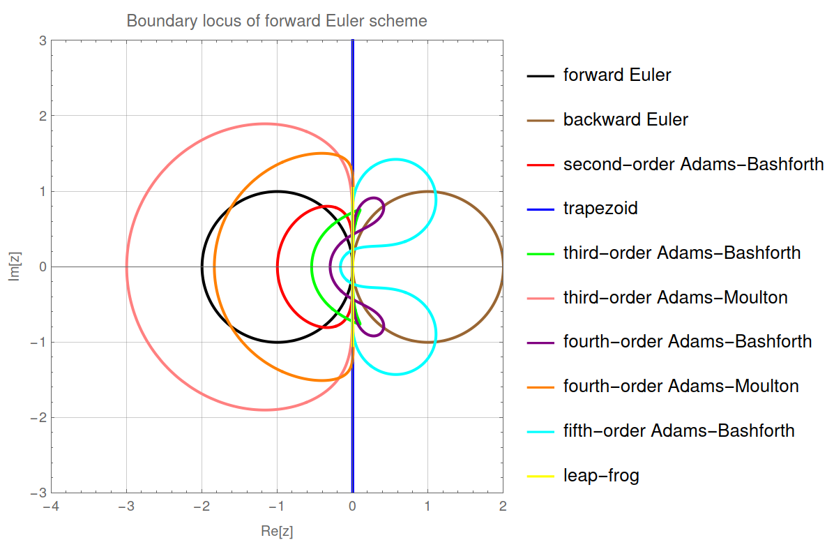
A method is said to be -stable if its region of stability contains the entire left half-plane in , and is said to be -stable if

Chapter 4
Nonlinear Operator Approximation

The null space of a linear mapping represented through matrix is defined as , the set of all points that have a null image through the mapping. The null space is a vector subspace of the domain of the linear mapping. A first step in the study of nonlinear mappings is to consider the generalization of the concept of a null set, starting with the simplest case,

where , , , i.e., has continuous derivatives. It is assumed that a closed form analytical solution is not available, and algorithms are sought to construct an approximating sequence whose limit is a root of (). The general approach is to replace () with

where is some approximation of , and the root of () can be easily determined.

Consider (a linear function, but not a linear mapping for ), an approximant of based upon data , given in Newton interpolant form by

The solution of () is

x_{n} = x_{n - 2} - \frac{f_{n - 2}}{f_{n - 1} - f_{n - 2}} (x_{n - 1} - x_{n - 2}) = \frac{x_{n - 2} f_{n - 1} - x_{n - 1} f_{n - 2}}{f_{n - 1} - f_{n - 2}},

an iteration known as the secant method. The error in root approximation is

e_{n} = x_{n} - x = e_{n - 2} - \frac{f_{n - 2}}{f_{n - 1} - f_{n - 2}} (e_{n - 1} - e_{n - 2}),

and can be estimated by Taylor series expansions around the root for which ,

f_{n - k} = f (x_{n - k}) = f^{'} (x) (x_{n - k} - x) + \frac{1}{2} f^{''} (x) {(x_{n - k} - x)}^{2} + \dots = f^{'} e_{n - k} + \frac{1}{2} f^{''} e_{n - k}^{2} + \dots,

where derivatives are assumed to be evaluated at . In the result

e_{n} = e_{n - 2} - \frac{f^{'} e_{n - 2} + \frac{1}{2} f^{''} e_{n - 2}^{2} + \dots}{f^{'} \cdot (e_{n - 1} - e_{n - 2}) + \frac{1}{2} f^{''} \cdot (e_{n - 1}^{2} - e_{n - 2}^{2}) + \dots} (e_{n - 1} - e_{n - 2}) = e_{n - 2} [1 - \frac{f^{'} + \frac{1}{2} f^{''} \cdot e_{n - 2} + \dots}{f^{'} + \frac{1}{2} f^{''} \cdot (e_{n - 1} + e_{n - 2}) + \dots}],

assuming , (i.e., is a simple root) gives

e_{n} = e_{n - 2} [1 - \frac{1 + c \cdot e_{n - 2} + \dots}{1 + c \cdot (e_{n - 1} + e_{n - 2}) + \dots}], c = \frac{1}{2} (f^{''} / f^{'}) .

For small errors, to first order the above can be written as

e_{n} = e_{n - 2} [1 - (1 + c \cdot e_{n - 2}) (1 - c \cdot (e_{n - 1} + e_{n - 2}))] = c e_{n - 1} e_{n - 2} .

Assuming -order convergence of ,

| e_{n} | \sim A {| e_{n - 1} |}^{p},

leads to

A^{p + 1} {| e_{n - 2} |}^{p^{2}} \sim c A {| e_{n - 2} |}^{p + 1} \Rightarrow {| e_{n - 2} |}^{p^{2} - p - 1} \sim c A^{- p} .

Since are finite while , the above asymptotic relation can only be satisfied if

p^{2} - p - 1 = 0 \Rightarrow p = \frac{1 + \sqrt{5}}{2} ≅ 1.62,

hence the secant method exhibits superlinear, but subquadratic convergence.

A different linear approximant arises from the Hermite interpolant based on data

{(x_{n - 1}, f_{n - 1} = f (x_{n - 1}), f_{n - 1}^{'} = f^{'} (x_{n - 1}))},

which is given in Newton form as

g_{n} (x) = f_{n - 1} + f_{n - 1}^{'} \cdot (x - x_{n - 1}),

with root

an iteration known as the Newton-Raphson method. The error is given by

Taylor series exapnsion around the root gives for small ,

e_{n} = e_{n - 1} - \frac{f^{'} \cdot e_{n - 1} + \frac{1}{2} f^{''} \cdot e_{n - 1}^{2} + \dots}{f^{'} + f^{''} e_{n - 1} + \dots} = e_{n - 1} [1 - \frac{1 + c e_{n - 1} + \dots}{1 + 2 c e_{n - 1} + \dots}] \approx e_{n - 1} [1 - (1 + c e_{n - 1}) (1 - 2 c e_{n - 1})] .

The resulting expression

states quadratic convergence for Newton's method. This faster convergence than the secant method requires however knowledge of the derivative, and the computational expense of evaluating it.

The above estimate assumes convergence of , but this is not guaranteed in general. Newton's method requires an accurate initial approximation , within a neighborhood of the root in which is increasing, , and convex, . Equivalently, since roots of are also roots of , Newton's method converges when . In both cases () in the prior iteration states that , hence . Since is increasing , hence () implies . Thus the sequence is decreasing and bounded below by zero, hence , and Newton's method converges.

An immediate extension of the above approach is to increase the accuracy of the approximant by seeking a higher-degree polynomial interpolant. The expense of the resulting algorithm increases rapidly though, and in practice linear and quadratic approximants are the most widely used. Consider the Hermite interpolant based on data

{(x_{n - 1}, f_{n - 1} = f (x_{n - 1}), f_{n - 1}^{'} = f^{'} (x_{n - 1}),, f_{n - 1}^{''} = f^{''} (x_{n - 1}))},

given in Newton form as

g_{n} (x) = f_{n - 1} + f_{n - 1}^{'} \cdot (x - x_{n - 1}) + \frac{1}{2} f_{n - 1}^{''} \cdot {(x - x_{n - 1})}^{2} = C + B s + A s^{2},

with roots

x_{n} = x_{n - 1} + \frac{- f_{n - 1}^{'} \pm \sqrt{{(f_{n - 1}^{'})}^{2} - 2 f_{n - 1} f_{n - 1}^{''}}}{f_{n - 1}^{''}} .

Tha above exhibits the difficulties arising in higher-order interpolants. The iteration requires evaluation of a square root, and checking for a positive discriminant.

Algebraic manipulations can avoid the appearance of radicals in a root-finding iteration. As an example, Halley's method

x_{n} = x_{n - 1} - \frac{2 f_{n - 1} f_{n - 1}^{'}}{2 {(f_{n - 1}^{'})}^{2} - f_{n - 1} f_{n - 1}^{''}},

exhibits cubic convergence.

The secant iteration

x_{n} = x_{n - 2} - \frac{f_{n - 2}}{f_{n - 1} - f_{n - 2}} (x_{n - 1} - x_{n - 2}) = x_{n - 2} - f_{n - 2},

in the limit of recovers Newton's method

x_{n} = x_{n - 1} - \frac{f_{n - 1}}{f_{n - 1}^{'}} .

This suggests seeking advantageous approximations of the derivative

x_{n} = x_{n - 1} - f_{n - 1},

based upon some step-size sequence . Since , the choice suggests itself, leading to Steffensen's method

x_{n} = x_{n - 1} - f_{n - 1} = x_{n - 1} - \frac{f_{n - 1}}{g_{n - 1}}, g_{n - 1} = - 1 .

Steffensen's method exhibits quadratic convergence, just like Newton's method, but does not require knowledge of the derivative. The higher order by comparison to the secant method is a direct result of the derivative approximation

f^{'} (x_{n - 1}) ≅,

which, remarkably, utilizes a composite approximation

f (x_{n - 1} + f (x_{n - 1})) = (f \circ (1 + f)) (x_{n - 1}) .

Such composite techniques are a prominent feature of various nonlinear approximations such as a -layer deep neural network .

The above iterative sequences have the form

x_{n} = F (x_{n - 1}),

and the root is a fixed point of the iteration

x = F (x) .

For example, in Newton's method

F (x) = x - \frac{f (x)}{f^{'} (x)},

and indeed at a root . Characterization of mappings that lead to convergent approximation sequences is of interest and leads to the following definition and theorem.

The fixed point theorem is an entry point to the study of non-additive approximation sequences.

Consider now nonlinear finite-dimensional mappings , and the root-finding problem

whose set of solutions generalize the linear mapping concept of a null space, . As in the scalar-valued case, algorithms are sought to construct an approximating sequence whose limit is a root of (), by approximating with , and solving

Multivariate approximation is however considerably more complex than univariate approximation. For example, consider , , and the univariate monomial interpolants in Lagrange form

ℒ_{t} 𝒇 (s, t) = \sum_{i = 0}^{m} 𝒇 (x_{i}, t) l_{i}^{x} (s), ℒ_{s} 𝒇 (s, t) = \sum_{j = 0}^{n} 𝒇 (s, y_{j}) l_{j}^{y} (t),

with

l_{i}^{x} (s) = \prod_{k = 0}^{m}^{'} \frac{s - x_{k}}{x_{i} - x_{k}}, l_{j}^{y} (s) = \prod_{l = 0}^{n}^{'} \frac{t - y_{l}}{y_{j} - y_{l}} .

The operator carries out interpolation at fixed value of the data set . Similarly, operator carries out interpolation at fixed value of the data set . Multivariate interpolation of the data set

𝒟 = {(x_{i}, y_{j}, 𝒇 (x_{i}, y_{j})), i = 0, \dots, m, j = 0, \dots, n},

can be carried out through multiple operator composition procedures.

Operator product: Define as
$ℒ 𝒇 (s, t) = (ℒ_{t} ℒ_{s}) 𝒇 (s, t) = ℒ_{t} (ℒ_{s} 𝒇 (s, t)) = ℒ_{t} (\sum_{i = 0}^{m} 𝒇 (x_{i}, t) l_{i}^{x} (s)) = \sum_{i = 0}^{m} \sum_{j = 0}^{n} 𝒇 (x_{i}, y_{j}) l_{i}^{x} (s) l_{j}^{y} (t) .$
Operator Boolean sum: Define as
$ℒ 𝒇 (s, t) = \sum_{i = 0}^{m} 𝒇 (x_{i}, t) l_{i}^{x} (s) + \sum_{j = 0}^{n} 𝒇 (s, y_{j}) l_{j}^{y} (t) - \sum_{i = 0}^{m} \sum_{j = 0}^{n} 𝒇 (x_{i}, y_{j}) l_{i}^{x} (s) l_{j}^{y} (t) .$

Bivariate () root-finding algorithms already exemplify the additional complexity in constructing root finding algorithms. The goal is to determine a new approximation from the prior approximants

(x_{0}, y_{0}), \dots, (x_{k - 2}, y_{k - 2}), (x_{k - 1}, y_{k - 1}) .

Whereas in the scalar case two prior points allowed construction of a linear approximant, the two points in data

𝒟 = {(x_{k - 2}, y_{k - 2}), (x_{k - 1}, y_{k - 1})}

are insufficient to determine

ℒ 𝒇 = \sum_{i = k - 2}^{k - 1} \sum_{j = k - 2}^{k - 1} 𝒇 (x_{i}, y_{j}) l_{i}^{x} (s) l_{j}^{y} (t),

which requires four data points. Various approaches to exploit the additional degrees of freedom are available, of which the class of quasi-Newton methods finds widespread applicability.

A linear multivariate approximant in dimensions requires data. A Hermite interpolant based upon function and partial derivative values can be constructed, but it is more direct to truncate the multivariate Taylor series

𝒇 (𝒙) = 𝒇 (𝒙_{k}) + \frac{\partial 𝒇}{\partial 𝒙} (𝒙_{k}) (𝒙 - 𝒙_{k}) + \dots,

where

𝑱 = \frac{\partial 𝒇}{\partial 𝒙} = [\begin{array}{llll} \frac{\partial f_{1}}{\partial x_{1}} & \frac{\partial f_{1}}{\partial x_{2}} & \dots & \frac{\partial f_{1}}{\partial x_{d}} \\ \frac{\partial f_{2}}{\partial x_{1}} & \frac{\partial f_{2}}{\partial x_{2}} & \dots & \frac{\partial f_{2}}{\partial x_{d}} \\ ⋮ & ⋮ & ⋱ \\ \frac{\partial f_{d}}{\partial x_{1}} & \frac{\partial f_{d}}{\partial x_{2}} & \dots & \frac{\partial f_{d}}{\partial x_{d}} \end{array}] = \nabla 𝒇,

is the Jacobian matrix of . Setting , as the condition for the next iterate leads to the update

𝑱 (𝒙_{k}) (𝒙_{k + 1} - 𝒙_{k}) = - 𝒇 (𝒙_{k}),

a linear system that is solved at each iteration. Computation of the multiple partial derivatives arising in the Jacobian might not be possible or too expensive, hence approximations are sought , similar in principle to the approximation of a tangent by a secant. In such quasi-Newton methods, a secant condition on is stated as

𝑩_{k} (𝒙_{k} - 𝒙_{k - 1}) = 𝒇 (𝒙_{k}) - 𝒇 (𝒙_{k - 1}),

and corresponds to a truncation of the Taylor series expansion around . The above secant condition is not sufficient by itself to determine , hence additional considerations can be imposed.

Recalling that the scalar Newton method for finding roots of converges in a region where , imposing analogous behavior for suggests itself. This is typically done by requiring to be symmetric positive definite.
Assuming convergence of the approximating sequence to a root, should be close to the previous approximation suggesting the condtion
${min}_{𝑩_{k + 1}} || 𝑩_{k + 1} - 𝑩_{k} || .$
Various algorithms arise from a particular choice of norm and procedure to apply ().

One widely used quasi-Newton method, arising from a rank-two update at each iteration to maintain positive definiteness, is the Broyden-Fletcher-Goldfard-Shanno update

𝑩_{k + 1} = 𝑩_{k} + \frac{𝒚_{k} 𝒚_{k}^{T}}{𝒚_{k}^{T} 𝒔_{k}} - \frac{𝑩_{k} 𝒔_{k} 𝒔_{k}^{T} 𝑩_{k}^{T}}{𝒔_{k}^{T} 𝑩_{k} 𝒔_{k}},

where the updates are determined by

Solving to find a search direction ;
Finding the distance along the search direction by ;
Updating the approximation ,
Computing .

All of the approximation techniques presented so far have been based upon linear approximation. For example, the polynomial interpolant

p_{m} (t) = a_{0} + a_{1} t + \dots + a_{m} t^{m}

of function based upon data set is linear in the unkown coefficients . A topic of current research is the development of nonlinear approximation procedures, for instance an approximation of by

f (t) ≅ g (t, 𝒂),

where is nonlinear in the parameters . Whereas the fundamental theorem of linear algebra completely characterizes linear approximants, there is currently no complete theory of nonlinear approximants. This leads to the ubiquity of heuristic techniques such as the mimicking of biological neurons that leads to artificial neuron approximants. The moniker of “machine learning” has been associated with adoption of such techniques, though the field is perhaps more insightfully seen as a natural development of linear approximants to consideration of nonlinear approximants.

The appearance of heuristic solution techniques in nonlinear approximation is typical of exploration of new mathematical fields. An instructive comparable development is the refinement of the formal rules of Heaviside operator calculus into a complete theory of distributions after some six decades of mathematical research.

In late nineteenth century, telegrapher's equations, a system of linear PDEs for current and voltage

\frac{\partial}{\partial x} V (x, t) = - L \frac{\partial}{\partial t} I (x, t) - R I (x, t)

\frac{\partial}{\partial x} I (x, t) = - C \frac{\partial}{\partial t} C (x, t) - G V (x, t)

Heaviside avoided solution of the PDEs by reduction to an algebraic formulation historical formulation, e.g., for the ODE for

\frac{d y}{d t} + a y = b

Heaviside considered the associated algebraic problem for

s Y + a Y = b \Rightarrow Y (s) = \frac{b}{a + s} \Rightarrow y (t) = ℒ^{- 1} [Y (s)]

Heaviside's formal framework (1890's) for solving ODEs was discounted since it lacked mathematical rigour.

Russian mathematician 1920's established first results (Vladimirov)
Theory of Distributions (Schwartz, 1950s)

Consider function , assumed large, of unknown form, difficult to compute for general input. Seek , such that

|| f - g \circ T || < ε

for some .

Choose a basis set (Monomials, Exponentials, Wavelets) to approximation of functions in Hibert space

g_{n} (t) = \sum_{j = 1}^{n} (f, ϕ_{j}) ϕ_{j} = \sum_{j = 1}^{n} c_{j} ϕ_{j}

The approximation is convergent if

{lim}_{n \to \infty} || f - g \circ T || = 0,

This assumes rapidly decrease.

Bessel inequality:

\sum_{j = 1}^{n} {| (f, ϕ_{j}) |}^{2} ⩽ {|| f ||}_{2} .

Fourier coefficient decay: for , absolutely continuous,

| c_{n} | ⩽ {min}_{0 ⩽ j ⩽ k} \frac{{|| f^{(j)} ||}_{1}}{{| n |}^{j}} .

In practice: coefficients decay as

for functions with discontinuities on a set of Lebesgue measure 0;
for functions with discontinuous first derivative on a set of Lebesgue measure 0;
for functions with discontinuous second derivative on a set of Lebesgue measure 0.

Fourier coefficients for analytic functions decay faster than any monomial power , a property known as exponential convergence.

Denote such approximations by , and they are linear

ℒ (α f + β g) = α ℒ (f) + β ℒ (g)

Choose a basis set (Monomials, Exponentials, Wavelets) to approximation of functions in Hibert space

g_{n} (t) = \sum_{j = 1}^{n} c_{j} ϕ_{j}

Let such

(f, φ_{k (1)}) ⩾ (f, φ_{k (2)}) ⩾ \dots ⩾ (f, φ_{k (n)}) .

Choose =, and

g_{n} (t) = \sum_{j = 1}^{n} c_{j} ϕ_{j} .

Denote such approximations by , and they are non-linear.

Consider function , assumed large, of unknown form, difficult to compute for general input. Seek , such that

|| f - g \circ T || < ε

for some .

What questions do you ask?

Does

Can arbitrary be achieved?

Can we construct

By what procedure?
$T = T_{1} \circ T_{2} \circ \dots \circ T_{J}$
with simple modifications of identity (ReLU)
${min}_{T_{1}, \dots T_{J}} || f - g \circ T_{1} \circ T_{2} \circ \dots \circ T_{J} ||$ $𝑻_{j} (𝒙) = η (𝑨_{j} 𝒙 + 𝒃_{j})$ $η (t) = {\begin{cases} 0 & t < 0 \\ t & t ⩾ 0 \end{cases} .$
At what cost?

How big is

Chapter 5
Differential Conservation Laws

Efficient algorithms often arise from the specifities of an underlying application domain, perhaps none more so than those inspired from physics. Classical physics can be derived from a remarkably small set of experimentally verified postulates.

The least action principle asserts that a physical system can be described by a function of the system generalized coordinates and velocities , known as the Lagrangian, itself the difference of the system's kinetic and potential energy . The time evolution of the system is known as the system's trajectory , and of all possible trajectories consistent with system constraints the trajectory actually followed by the system from initial time to final time minimizes a functional known as the action
$S (q, \dot{q}) = \int_{t_{0}}^{t_{1}} L (t, q (t), \dot{q} (t)) d t .$
One class of constraints are the conservation laws, the experimental observation that certain quantities remain constant during the system's evolution. Classical mechanics identifies three conserved quantities: mass, momentum, and energy. It is a matter of personal preference to also consider conservation of angular momentum as fundamental or as a consequence of conservation of linear momentum. Classical electrodynamics adds conservation of electric charge, while quantum mechanics also defines conservation of certain microscopic quantities known as quantum numbers such as the baryon or lepton numbers.

Other constraints often refer to allowed spatial positions and are known generically as geometric constraints. Note that this is an idealization: in reality some other physical system is interacting with the one being considered and it is assumed that the system is so much larger that its position does not change. Such idealization or modeling assumptions are often encountered. As another important example, the system may exhibit energy dissipation, such as the decrease of an object's momentum due to friction. Energy is indeed lost from system to the surrounding medium , but the overall energy of the combined system is conserved.

Scientific computation uses many concepts and terms from physics, such as the characterization of a numerical scheme for differential equations as being “conservative”, in the sense of maintaining the conserved physical quantities. Also, a remarkably large number of efficient algorithms arise from the desire to mimic physical properties. Conservation laws can be stated for a small enough spatial domain that it can be considered to be infinitesimal in the sense of calculus. In this case differential conservation laws are obtained. Alternatively, consideration of a finite-sized spatial domain leads to integral formulation of the conservation laws. In a large class of physical systems of current research interest models are constructed in which the evolution of the system depends on the history of interactions with the surrounding medium . Such systems are described by integro-differential laws, elegantly expressed through fractional derivatives.

Conservation of some physical quantity is stated for a hypothesized isolated system. In reality no system is truly isolated and the most interesting applications come about from the study of interaction between two or more systems. This leads to the question of how one can follow the changes in physical quantities of the separate systems. An extremely useful procedure is to set up an accounting procedure. A mundane but illuminating example is quantity of Euros in a building . If the building is a commonplace one, it is to be expected that when completely isolated, the amount of currency in the building is fixed

is some constant. Equation () is self-evident but not particularly illuminating – of course the amount of money is constant if nothing goes in or out! Similar physics statements such as “the total mass-energy of the universe is constant” are again not terribly useful, though one should note this particular statement is not obviously true. Things get more interesting when we consider a more realistic scenario in which the system is not isolated. People might be coming and going from building and some might actually have money in their pockets. In more leisurely economic times, one might be interested just in the amount of money in the building at the end of the day. Just a bit of thought leads to

E_{n} = E_{n - 1} + Δ E_{n - 1, n}

where is the amount of money at the end of day , that from the previous day and the difference between money received and that payed in the building during day

Δ E_{n - 1, n} = R_{n - 1, n} - P_{n - 1, n} .

As economic activity picks up and we take building to mean “bank” it becomes important to keep track of the money at all times, not just at the end of the day. It then makes sense to think of the rate at which money is moving in or out of the building so we can not only track the amount of currency at any given time, but also be able to make future predictions. Instead of separate receipts and payments , use a single quantity to denote the amount of money leaving or entering building during time interval with the understanding that positive values of represent incomes and negative ones expenditures. Such understandings go by the name of sign conventions. They're not especially meaningful but it aids communication if a single convention is adopted. The amount of euros in the building then changes in accordance to

and is known as a flux, the Latin term for flow.

While () is a good approximation for small intervals, errors arise when is large since economic acitvity might change from hour to hour. Better accounting is obtained by considering as defined at any given time , such that is the instantaneous flux of euros at time . The fundamental theorem of calculus then states

with the same significance as ().

In a large bank one keeps track of the amount of money in individual rooms and the inflows and outflows through individual doors. A room or door can be identified by its spatial position , but refers to a single point and physical currency occupies some space. The conceptual difficulty is overcome by introducing a fictitious density of currency at time denoted by . The only real meaning associated with this density is that the sum of all values of in some volume is the amount of currency in that volume

On afterthought, the same sort of question should have arisen when was defined at one instant in time. Ingrained psychological perspectives make more plausible, but were we to live our lives such that quantum fluctuations are observable, would be much more questionable.

By an analogous procedure, define as the instantaneous flux density of euros in a small region around . This flux is a vector quantity to distinguish fluxes along different spatial directions. The flux density along direction is given by . Consider as the inward pointing unit vector normal to the surface that bounds the bank. The total flux is again obtained by integrating flux densities

Gathering the above leads to re-expressing () or () gives

Using () leads to the statement,

\int_{B} e (𝒙, t + Δ t) d 𝒙 = \int_{B} e (𝒙, t) d 𝒙 + \int_{t}^{t + Δ t} \int_{\partial B} 𝒇 (𝒙, τ) \cdot 𝒏 (𝒙) d 𝒙 d τ .

There are special cases in which additional events affecting the balance of can occur. When is a reserve bank money might be (legally) printed and destroyed in the building. Again by analogy with fluid dynamics, such events are said to be sources of within , much like a underground spring is a source of surface water. Let be the total sources at time . As before, might actually be obtained by summing over several sources placed in a number of positions, for instance the separate printing presses and furnaces that exist in . It is useful to introduce a spatial density of sources . The conservation statement now becomes

The above encompasses all physical conservation laws, and is quite straightforward in interpretation:

It should be emphasized that the above statement has true physical meaning and is referred to as an integral formulation of a conservation law. The key term is “integral” and refers to the integration over some spatial domain.

Equation () is useful and often applied directly in the analysis of physical systems. From an operational point of view it does have some inconveniences though. These have mainly to do with the integration domains , sometimes difficult to describe and to perform integrations over. Avoid this by considering defined everywhere, not only on (the doors and windows of ). These internal fluxes can be shown to have a proper physical interpretation. Assuming that is smooth allows use of the Gauss theorem to transform the surface integral over into a volume integral over

The minus assign arises from the convention of an inward pointing normal. Applying () to () leads to

There was nothing special about the shape of the building or the length of the time interval we used in deriving (), hence the equality should hold for infinitesimal domains

where, as is customary, the dependence of on space and time is understood but not written out explicitly. Equation () is known as the local or differential form of the conservation law for .

The full general form () often arises in applications, but simplifications can arise from specific system properties. As a simple example, the dynamics of a point mass which has no internal structure is described by the conservation of momentum statement

The correspondence with () is given by , , hence the statement: “external forces are sources of momentum”. Instead of a PDE, the lack of internal structure has led to an ODE.

Other special forms of () are not quite so trivial. Often depend on , with the specific form of this dependence is given by physical analysis. Accounting for all physical effects is so difficult that simple approximations are often used. For instance if is sufficiently smooth Taylor series expansion gives

Choosing the origin such that and , the simplest truncation is

and the form of () is

In this approximation is a constant giving

known as the constant velocity advection equation. Its one-dimensional form is the basis of much development in numerical methods for PDE's

Another widely encountered dependence of on is of the form

and this leads to

If there are no sources and is a constant we have

the heat or diffusion equation.

Both above flux types can appear in which case the associated conservation law is

known as the advection-diffusion equation, and is a linear PDE. If sources exist the above becomes

or for constant advection velocity

It is often the case that the flux depends on the conserved quantity itself, , in which case () becomes a non-linear PDE.

Various effects can balance leading to no observable time dependence, . If there is no overall diffusive flux within an infinitesimal volume, then leads to the Laplace equation

\nabla^{2} e = 0 .

If the infinitesimal volume contains sources the Poisson equation

\nabla^{2} e = σ,

is obtained.

Often, the time dependence can be isolated from the spatial dependence, , in which case the diffusion equation for constant leads to

\frac{\dot{T}}{T} = α \frac{\nabla^{2} X}{X} = - λ,

with a positive constant to avoid unphysical exponential growth. The spatial part of the solution statisfies the Helmholtz equation

\nabla^{2} X = - κ^{2} X,

with . The above is interpreted as an eigenproblem for the Laplacian operator .

The above special forms of differential conservation laws play an important role in scientific computation. Numerical techniques have been developed to capture the underlying physical behavior expressed in say the diffusion equation or the Helmholtz equation. These equations were first studied within physics, but they reflect universal behavior. Consider the Black-Scholes financial model for the price of an option on an asset

\frac{\partial V}{\partial t} + r S \frac{\partial V}{\partial S} = r V - \frac{1}{2} σ^{2} S^{2} \frac{\partial^{2} V}{\partial S^{2}},

with the standard deviation of stock market returns and the annualized risk-free interest rate. The terminology might be totally different, but the same patterns emerge and the Black Scholes model can be interpreted as an advection diffusion equation with non-constant advection velocity , negative diffusion coefficient and source term . The similarity to the physics advection and diffusion equations arises from the same type of modeling assumptions relating fluxes to state variables.

A first example of problem-specific algorithms is afforded by consideration of the steady-state diffusion problem

where can be understood to denote the temperature in an infinitesimal volume positioned at in -dimensional space, and is a local rate of heat generation. The above arises from setting the time derivative zero in . Though often stated in this thermal language, the Poisson equation () is generally valid for unresolved transport by Brownian motion. The mathematical concept of an “infinitesimal volume” is interpreted as setting some length scale much smaller than the length scale characterizing the size of the domain . As an example, for heat conduction in a column of water of length m the length scale of a quasi-infinitesimal volume can be considered as, say, m. There is no physical significance to the mathematical limit process due to the discrete structure of matter, and for all practical purposes setting m is an acceptable threshold to delimit a phenomenon of interest to behavior that can be neglected. In this case the phenomenon of interest is the average transport of thermal energy in volumes of size greater than . The detailed Brownian motion of the water molecules that occurs on length scales can be neglected and is said to be unresolved. The only observable effect of this motion is that temperature gradients lead to a heat flux as described by (Fourier's law). The same equation () arises in epidemiology when m, an average separation between an infected and susceptible individual, , the size of a large city, and is reinterpreted as the percentage of infected individuals in the population. Again, the detailed Brownian steps of size taken by individuals can be neglected.

Understanding the underlying unresolved Brownian motion is useful in constructing numerical solutions. For , () becomes which states that there is no net heat flux in an infinitesimal volume, , colloquially: “what flows in on one side goes out on the other”. A function that satisfies Laplace's equation is said to be harmonic. For , the ordinary differential equation is obtained with solution , and boundary conditions at and at gives . A temperature difference at the boundaries induces diffusive fluxes that lead to the mean value at the midpoint. An analogous statement is made for starting from Green's formula on ball with spherical boundary of radius

\int_{B} (u Δ v - v Δ u) d ω = \int_{S = \partial B} (u \frac{\partial v}{\partial n} - v \frac{\partial u}{\partial n}) d σ,

for scalar functions . For and the mean value theorem

is obtained, which states that the value of a harmonic function is the average of the values on a surrounding sphere. For the analogous statement is

Midpoint quadrature of () over four subintervals gives

Apply the above on a grid covering some arbitrary domain with boundary to obtain

Complications arise for general boundaries , but for a square domain grid points align with the boundary, . Instead of two indices, one for each spatial direction, organize the grid values through a single index , with denoting the value at the interior points . The vector of interior grid values has components, and the mean value theorem leads to the linear system

where has a regular sparsity pattern induced by the uniform spacing of the grid

𝑨 = [\begin{array}{llllllllll} 4 & - 1 & 0 & \dots & 0 & - 1 & 0 & \dots & \dots & 0 \\ - 1 & 4 & - 1 & 0 & \dots & 0 & - 1 & 0 & \dots & 0 \\ ⋱ & ⋱ & ⋱ & ⋱ \end{array}] .

The vector contains the boundary values, for example .

The system () was obtained by discretization of the mean-value integral (). The same linear system is also obtained by discretization of the differential equation

- \nabla^{2} u = - u_{x x} - u_{y y} = 0,

where indices denote differentiation. The minus sign arises from compatibility with the unsteady form of the heat equation . A centered finite difference approximation of the derivatives on the uniform grid leads to

u_{x x} (x_{i}, y_{j}) ≅ \frac{u_{i - 1, j} - 2 u_{i, j} + u_{i + 1, j}}{h^{2}}, u_{y y} (x_{i}, y_{j}) ≅ \frac{u_{i, j - 1} - 2 u_{i, j} + u_{i, j + 1}}{h^{2}},

and () is recovered. For the Poisson equation the right hand side changes to

with . It is often the case that the same discrete system arises from both the differential and the integral formulation of a conservation law on a uniform grid.

The above discussion of the underlying physics of the Poisson equation productively guides construction of numerical solution procedures. Solving the linear system () by general factorizations such as or is costly in terms of memory usage since the sparisty pattern is lost. For the uniform grid and square domain considered above the matrix need not be explicitly stored at all since , and when or . The discrete mean value theorem () suggests that some approximation can be improved by the iteration

The above is known as Jacobi iteration, and can be stated in matrix form by expressing as

with containing non-zero components of below, above the diagonal, and containing the diagonal of . In contrast to the multiplicative decompositions considered up to now, the , , SVD, eigen or Schur decompositions, the decomposition () is now additive. Note that in () are strictly lower, upper diagonal matrices with zeros on the diagonal in contrast to the notation for the standard factorization algorithm. Recall that the utility of matrix multiplication was associated with the representation of linear mapping composition. Additive decompositions such as () generally are useful when separating different aspects of a physical process, and are a simple example of operator splitting. For the discrete Poisson system Jacobi iteration can be expressed as

Several variants of the idea can be pursued. The matrix splitting () is useful in theoretical convergence analysis, but implementations directly use () within loops over the indices. Updated values can be immediately utilized leading to either of the following iterations

depending on loop organization. These are known as Gauss-Seidel iterations. Convergence might accelerated by extrapolation,

where the new iteration is continued by factor in the direction of the Gauss-Seidel update. When this is known as successive over-relaxation (SOR) and goes further in the Gauss-Seidel direction. Choosing leads to successive under-relaxation.

Turning now from algorithm construction to analysis of its behavior, simplify notation by letting denote the current iterate. The previous notation was convenient since individual components were referenced as in , but convergence analysis is determined by the properties of the operator splitting and not of the current iterate. Introduce the error at iteration as the difference between the exact solution and the current iterate , . Also introduce the residual , and the correction to the current iterate

The above methods can be formulated as a residual correction algorithm through the steps:

residual computation,
correction computation,
approximation update,

When the exact solution is recovered in one step

𝒆_{k} = 𝑨^{- 1} (𝒄 - 𝑨 𝒖_{k}) = 𝒖 - 𝒖_{k} \Rightarrow 𝒖_{k + 1} = 𝒖_{k} + 𝒆_{k} = 𝒖 .

Iterative methods use some approximation of the (unknown) inverse, . Jacobi iteration uses since

𝒖_{k + 1} = 𝒖_{k} + 𝑫^{- 1} [𝒄 - (𝑳 + 𝑫 + 𝑼) 𝒖_{k}] = 𝑫^{- 1} [𝒄 - (𝑳 + 𝑼) 𝒖_{k}],

recovering (). Table shows several common choices for . Two key aspects govern the choice of the inverse approximant:

Computational efficiency stated as a requirement that each iteration cost either or operations;
Capturing the essential aspects of .

The iteration converges to the solution if for increasing . The error at iteration is expressed as

The repeated matrix multiplication indicates that the eigenstructure of the iteration matrix determines iteration convergence. Indeed the above is simply power iteration for and can be expected to converge as

𝜹_{k} \to μ_{1}^{k} c_{1} 𝒒_{1},

with the eigenpair that corresponds to the largest eigenvalue in absolute value, , known as the spectral radius of , denoted by Clearly, the above iterations will exhibit linear order of convergence when . The rate of convergence at iteration is estimated by the Rayleigh quotient

s_{k} = \frac{𝜹_{k}^{T} 𝑴 𝜹_{k}}{𝜹_{k}^{T} 𝜹_{k}} = \frac{𝜹_{k}^{T} 𝜹_{k + 1}}{𝜹_{k}^{T} 𝜹_{k}},

and is monitored in implementations of iterative methods, and determined by the eigenvalues of .

The eigenstructure of is difficult for arbitrary matrices , but can be carried out when has special structure induced by known physical phenomena. The relation between analytical and numerical formulations plays an essential role in convergence analysis. The diffusion equation () leads to a symmetric matrix , due to two aspects:

the chosen discretization is symmetric using centered finite differences;
the operator itself exhibits symmetry.

Insight into the above two aspects is most readily gained from the one-dimensional case with homogeneous Dirichlet boundary conditions . The linear system obtained from the centered finite difference discretization

- u_{i - 1} + 2 u_{i} - u_{i + 1} = h^{2} f_{i}, i = 1, \dots, m, h = 1 / (m + 1), u_{0} = u_{m + 1} = 0,

has a symmetric tridiagonal system matrix . The symmetry can be expressed through scalar products in a way that generalizes to differential operators. Recall that a real-valued scalar product must satisfy symmetry . For the standard inner product has this property. Consider the action of the operator on the two terms. If the operator is said to be symmetric. For the inner product

(𝑨 𝒖, 𝒗) = {(𝑨 𝒖)}^{T} 𝒗 = 𝒖^{T} 𝑨^{T} 𝒗, (𝒖, 𝑨 𝒗) = 𝒖^{T} 𝑨 𝒗,

and the two expressions are equal if . The same approach extends to the diffusion operator using the scalar product

(f, g) = \int_{0}^{1} f (x) g (x) d x .

Applying integration by parts

(\partial_{x x} f, g) = \int_{0}^{1} f^{''} (x) g (x) d x = {[f^{'} g]}_{x = 0}^{x = 1} - \int_{0}^{1} f^{'} (x) g^{'} (x) d x = {[f^{'} g]}_{x = 0}^{x = 1} - {[f g^{'}]}_{x = 0}^{x = 1} + \int_{0}^{1} f (x) g^{''} (x) d x = b + (f, \partial_{x x} g) .

For homogeneous boundary conditions , the symmetry condition is satisfied. Note that symmetry involves both the operator anId the boundary conditions of the problem. For the scalar product

(u, v) = \int_{Ω} u (x, y) v (x, y) d x d y,

is defined on the unit square , and for homogeneous Dirichlet boundary conditions two applications of Green's formula leads to , and the Laplace operator is symmetric.

For , , , the eigenvalues of are inferred from those of the operator with homogeneous boundary conditions at ,

- \partial_{x x} \sin (κ π x) = {(κ π)}^{2} \sin (κ π x), κ \in ℕ .

Positing that an eigenvector of is the discretization of the continuum eigenfunction leads to

q_{j} = \sin (κ π x_{j}) = \sin (κ π j h) = \sin (\frac{j κ π}{m + 1}),

hypothesis that is verified by the calculation of component of

{(𝑨 𝒒)}_{j} = - \sin [\frac{(j - 1) κ π}{m + 1}] + 2 \sin [\frac{j κ π}{m + 1}] - \sin [\frac{(j + 1) κ π}{m + 1}] = 2 [1 - \cos (\frac{κ π}{m + 1})] \sin (\frac{j κ π}{m + 1}),

thereby obtaining the eigenvalue

v_{κ} = 2 [1 - \cos (\frac{κ π}{m + 1})] = 4 \sin^{2} [\frac{κ π h}{2}],

which recovers the analytical eigenvalue in the limit

{lim}_{h \to 0} \frac{v_{κ}}{h^{2}} = {(κ π)}^{2} .

For Jacobi , so the eigenvalues of are

λ_{κ} = 2 \sin^{2} [\frac{κ π h}{2}], κ = 1, 2, \dots, m .

The eigenvalues of are therefore

μ_{κ} = 1 - 2 \sin^{2} [\frac{κ π h}{2}] = \cos (κ π h)

Replacing the largest eigenvalue is obtained for

μ_{max} = μ_{1} = \cos (\frac{π}{m + 1}) .

For large , , and slow convergence is expected as verified in the numerical experiment from Fig. .

Jacobi iteration and its variants have limited practical utility by comparison to other iterative procedures due to slow convergence, but the concept of operator spliting has wide applicability. A more consequential example of operator splitting is to consider the advection diffusion equation

q_{t} + 𝒗 \cdot \nabla q = α Δ q,

which can be interpreted as stating that the time evolution of is due to the effect of a diffusion operator and an advection operator

q_{t} = (𝒜 + ℬ) q .

Suppose both operators are discretized leading to matrices and the discrete system

𝒒_{t} = (𝑨 + 𝑩) 𝒒,

with initial condition . Advancing the solution by a time step can be written as

𝒒 (t + Δ t) = e^{Δ t (𝑨 + 𝑩)} 𝒒 (t),

and can be separated into two stages

𝒒^{(l + 1)} = e^{Δ t 𝑨} e^{Δ t 𝑩} 𝒒^{(l)} .

The quantity captures advection effects and is the diffusion correction. Since advection and diffusion are markedly different physical effects describing resolved versus unresolved transport, it can be expected that matrices have different properties that require specific solution procedures.

By contrast, the Jacobi iteration splitting does not separate physical effects and simply is suggested by the sparsity of and computational efficiency per iteration. For example, the forward Gauss-Seidel iteration with leads to

The matrix is (non-strictly) lower-triangular and () is easily solved by forward substitution. The implementation is very simple to express while preserving two-dimensional indexing.

In the above implementation a single memory space is used for with new values taking place of the old, leading to just four floating point additions and one multiplication per grid point. Since the algorithm essentially takes the current average of neighboring values, it is also known as a relaxation method, smoothing out spatial variations in .

Though such simple implementation is desirable, the non-physical splitting and associated slow convergence usually outweighs ease of coding effort and suggests looking for alternative approaches. The only scenarios where such simply implemented iterations find practical use is in parallel execution and as a preliminary modification of the system prior to use of some other algorithm.

Alternatives to exploiting problem structure by operator splitting are suggested by the least action principle. The action

S (q, \dot{q}) = \int_{t_{0}}^{t_{1}} L (t, q (t), \dot{q} (t)) d t,

is a functional over the phase space of the system, e.g., for a system composed of point masses. The least action principle states that the observed trajectory minimizes the action, hence it is to be expected that optimization algorithms that solve the problem

{min}_{q, \dot{q}} S

would be of interest. This indeed is the case and leads to a class of methods that can exhibit remarkably fast convergence and more readily generalize to variable physical properties and arbitrary domain geometry.

A first step in considering linear operators that still exhibit structure but are more complex than the constant-coefficient discretization of the Laplacian is to consider spatially-varying diffusivity in which case the steady-state heat equation in domain becomes

again with Dirichlet boundary conditions on . Maintaining simple domain geometry for now, the centered finite-difference discretization of () on with grid points becomes

where denotes a diffusivity average at and contains the boundary conditions and forcing term as before, . The sparsity pattern is the same as in the constant diffusivity case, but the system has a system matrix with variable coefficients. The matrix expresses a self-adjoint operator through a symmetric discretization, namely centered finite differences on a uniform grid. It can be expected to be symmetric , as verified by considering row , that has non-zero components in columns , , . It is sufficient to verify symmetry for entries within the lower triangle of . The component is the coefficient of in () . Symmetry of would require . The component arises from row

- α_{i - 1 / 2, j} u_{i, j} - α_{i - 3 / 2, j} u_{i - 2, j} - α_{i - 1, j + 1 / 2} u_{i - 1, j + 1} - α_{i - 1, j - 1 / 2} u_{i - 1, j - 1} + 4 {\overline{α}}_{i - 1, j} u_{i - 1, j} = c_{i - 1, j} .

The diagonal element for row has indices and the column has indices for which , indeed verifying . Such opaque index manipulations can readily be avoided by symmetry considerations as stated above: self-adjoint operator expressed through symmetric discretization. The physical argument is even simpler. Diffusivity expresses how readily heat is transferred between two spatial positions of unequal temperature, and there is no reason for this material property to differ in considering the heat flux from point to point , from that from point to , . Setting to account for direction of heat flow leads to , and this material property is reflected in symmetry of . Note that even though the operator might be self-adjoint under appropriate boundary conditions, unsymmetric discretization such as one-sided finite differences can lead to a non-symmetric system matrix .

The implications for iterative method convergence can again be surmised from the one-dimensional case with homogeneous boundary conditions , . The convergence rate for an iterative method depends on the eigenvalues of the matrix obtained by discretization of the operator . The regular Sturm-Liouvile eigenproblem , is known to have a solution, albeit difficult to obtain analytically. Replacing analytical estimates by a numerical experiment taking , Fig. shows that convergence becomes marginally slower as the diffusivity gradient increases, though the main difficulty is the spectral radius for constant diffusivity.

The heat equation can be obtained as the stationary solution , to an optimization problem for the functional

among all functions that satisfy the boundary condition on . The above can be understood as the generalization of the one-dimensional case

Φ (u, u^{'}) = - \int_{0}^{1} (\frac{1}{2} α u^{'} u^{'} + u f) d x .

The stationarity condition point for is

δ Φ = - \int_{0}^{1} (α u^{'} δ u^{'} + f δ u) d x = - \int_{0}^{1} (α u^{'} \frac{d}{d x} δ u + f δ u) d x = - {[α u^{'} δ u]}_{x = 0}^{x = 1} + \int_{0}^{1} (\frac{d}{d x} (α u^{'}) - f) δ u d x = 0 .

Since all must satisfy boundary conditions the perturbations are null at endpoints , and stationarity for arbitrary perturbations implies that

\frac{d}{d x} (α u^{'}) - f = 0,

the one-dimensional variable diffusivity heat equation.

How can the above observations guide algorithm construction? The key point is that the discrete problem should also be expressible as an optimization problem for

Φ (𝒖) = \frac{1}{2} 𝒖^{T} 𝑨 𝒖 - 𝒖^{T} 𝒄 = \frac{1}{2} \sum_{j = 1}^{m} \sum_{k = 1}^{m} u_{j} a_{j k} u_{k} - \sum_{j = 1}^{m} u_{j} c_{j},

with . The discrete stationarity condition is leading to

\frac{\partial Φ}{\partial u_{l}} = \frac{1}{2} \sum_{j = 1}^{m} \sum_{k = 1}^{m} (δ_{l j} a_{j k} u_{k} + u_{j} a_{j k} δ_{l k}) - \sum_{j = 1}^{m} δ_{l j} c_{j} .

Using the Kronecker delta properties , for gives

\frac{\partial Φ}{\partial u_{l}} = \frac{1}{2} \sum_{k = 1}^{m} a_{l k} u_{k} + \frac{1}{2} \sum_{j = 1}^{m} u_{j} a_{j l} - c_{l},

which for symmetric leads to

Symmetric discretization of the self-adjoint operator produces a symmetric matrix that is unitarily diagonalizable , and, as seen previously, with strictly positive eigenvalues. Hence stationary points of are minima and the solution to can be sought by minimizing .

Equation () states that the gradient of is opposite the direction of the residual . Since this is the direction of fastest increase of , travel in the opposite direction will decrease leading to an update

of the current approximation . The correction direction is also referred to as a search direction for the optimization procedure. In the residual correction formulation

𝒓_{k} = 𝒄 - 𝑨 𝒖_{k}, 𝒆_{k} = 𝑩 𝒓_{k}, 𝒖_{k + 1} = 𝒖_{k} + 𝒆_{k},

steepest descent corresponds to the choice . The remaining question is to determine how far to travel along the search direction. As increases the local gradient direction changes. Steepest descent proceeds along the direction until further decrease is no longer possible, that is when the new gradient direction is orthogonal to the previous one

𝒓_{k}^{T} 𝒓_{k + 1} = 0 \Rightarrow 𝒓_{k}^{T} (𝒄 - 𝑨 𝒖_{k + 1}) = 𝒓_{k}^{T} [𝒄 - 𝑨 (𝒖_{k} + β_{k} 𝒓_{k})] = 𝒓_{k}^{T} (𝒓_{k} - β_{k} 𝑨 𝒓_{k}) = 0 \Rightarrow β_{k} = \frac{𝒓_{k}^{T} 𝒓_{k}}{𝒓_{k}^{T} 𝑨 𝒓_{k}} .

The convergence rate is given by the spectral radius of that becomes

𝑴 = 𝑰 - β_{k} 𝑨 = 𝑰 - \frac{𝒓_{k}^{T} 𝒓_{k}}{𝒓_{k}^{T} 𝑨 𝒓_{k}} 𝑨 .

Recall that the one-dimensional, constant diffusivity heat equation had eigenvalues of

v_{l} = 4 \sin^{2} [\frac{l π h}{2}], l = 1, 2, \dots, m .

Eigenvalues of gradient descent iteration are therefore

λ_{l} = 1 - β_{k} ν_{l}, l = 1, 2, \dots, m .

Since is the inverse of a Rayleigh quotient, if the residual is in the direction of eigenvector , and suggesting the possibility of fast convergence. However, the distribution of eigenvalues for is uniformly distributed in the interval [0,4] such that the residual component in other eigendirections is not significantly reduced. The typical behavior of gradient descent is rapid decrease of the residual in the first few iterations followed by slow convergence to the solution. Consider the problem

- u_{x x} = π^{2} \sum_{k = 1}^{K} k^{2} \sin (k π x), u (0) = u (1) = 0,

with solution

u (x) = \sum_{k = 1}^{K} \sin (k π x) .

The behavior of gradient descent is shown in Fig. . A good approximation of the solution shape is obtained after only a few gradient descent iterations, but convergence thereafter is slow.

Steepest descent is characterized by a correction in the direction of the residual (). Enforcing leads to orthogonality of both succesive residuals and correction directions. A more insightful interpretation of (3) is to recognize the role of the scalar products

(f, g) = \int_{Ω} α (\nabla f) \cdot (\nabla g) d 𝒙, (𝒖, 𝒗) = 𝒖^{T} 𝑨 𝒗,

in the continuum, discrete cases respectively. Similarly to how vectors that satisfy are said to be orthogonal, those that satisfy are said to be -conjugate. Gradient descent minimizes the 2-norm of the error at each iteration. However, the variational formulation suggests that a more appropriate norm is the -norm

{|| 𝒆_{k} ||}_{𝑨} = {(𝒆_{k}^{T} 𝑨 𝒆_{k})}^{1 / 2} .

This leads to a modification of the search directions , which are no longer taken in the direction of the residual and orthogonal, but rather -conjugate

𝒑_{k + 1}^{T} 𝑨 𝒑_{k} = 0 .

For the steady-state heat equation with spatially-varying diffusivity, symmetric discretizations on uniform grids lead to systems with , and a regular sparsity pattern. Irregular domain discretization will lead to more complicated sparsity patterns that require different approaches to solving the linear system. It is important to link the changes in the structure of to specific aspects of the approximation procedure. Consider the difficulties of applying finite difference discretization on a domain of arbitrary shape with boundary (Fig. ). At grid node closer to the boundary than the uniform spacing , centered finite difference formulas would refer to undefined values outside the domain. One-sided finite difference formulas would fail to take into account boundary values for the problem. Taylor series expansions could be used,

u_{A} = u (ξ h, j h) = u_{i, j} + {(\frac{\partial u}{\partial x})}_{i, j} (ξ h) + \frac{1}{2} {(\frac{\partial^{2} u}{\partial x^{2}})}_{i, j} {(ξ h)}^{2} + \dots

u_{_{i + 1, j}} = u_{i, j} + {(\frac{\partial u}{\partial x})}_{i, j} h + \frac{1}{2} {(\frac{\partial^{2} u}{\partial x^{2}})}_{i, j} h^{2} + \dots

from which elimination of the second derivative leads to an approximation of the first derivative as

Note that setting would place at a grid node, and from () the familiar centered finite difference approximation of the first derivative

{(\frac{\partial u}{\partial x})}_{i, j} = \frac{u_{i + 1, j} - u_{i - 1, j}}{2 h},

is recovered. For an arbitrary domain the values of would vary and the resulting linear system would no longer be symmetric. From a physical perspective this might be surprising at first since the operator is isotropic, but this is true for an inifinitesimal domain. Upon irregular discretization the problem is only an approximation of the physical problem , and can exhibit different behavior, in this case loss of isotropy near the boundaries.

Computing the appropriate mesh size fractions for all grid points near a boundary is an onerous task, and suggests seeking a different approach. A frutiful idea is to separate the problem of geometric description from that of physics expressed by some operator . Domains within of arbitrary complexity can be approximated to any desired precision by a simplicial covering. Simplicia are the simplest geometric objects with non-zero measure in a space. For these are line segments that can approximate arbitrary curves. The corresponding simplicia for and are triangles and tetrahedra, respectively. Consider and specify a set of triangles with vertices , , that form a partition of precision of the domain ,

\forall k, l \in {1, 2, \dots, n}, μ (T_{k} \cap T_{l}) = 0, | μ (⋃_{k = 1}^{n} T_{k}) - μ (Ω) | ⩽ ε .

The above state that intersections of triangles must have zero measure in , i.e., triangles can share edges or vertices but cannot overlap over a non-zero area. The area of the union of triangles approximates the area of the overall domain .

In a finite difference discretization the function is approximated by a set of values , often referred to as a grid function. Similarly, a set of values can be defined at the triangle vertices . Denote the vertex coordinates of triangle by , . Values of within the triangle are determined through piecewise interpolation, a generalization of one-dimensional -splines, using the form functions

N_{1} (x, y) = \frac{1}{2 A} | \begin{array}{lll} 1 & 1 & 1 \\ x & x_{2} & x_{3} \\ y & y_{2} & y_{3} \end{array} |, N_{2} (x, y) = \frac{1}{2 A} | \begin{array}{lll} 1 & 1 & 1 \\ x_{1} & x & x_{3} \\ y_{1} & y & y_{3} \end{array} |, N_{3} (x, y) = \frac{1}{2 A} | \begin{array}{lll} 1 & 1 & 1 \\ x_{1} & x_{2} & x \\ y_{1} & y_{2} & y \end{array} |,

with the triangle area

A = \frac{1}{2} | \begin{array}{lll} 1 & 1 & 1 \\ x_{1} & x_{2} & x_{3} \\ y_{1} & y_{2} & y_{3} \end{array} | .

Note that for the form functions give the fraction of the overall area occupied by the interior triangles such that . The linear spline interpolation of based upon the vertex values is

the familiar form of a linear combination. It is customary to set if , recovering the framework of -splines. Since thus approximated is non-zero only over the single triangle , such an approach is commonly referred to as a finite element method (FEM).

Various approaches can be applied to derive an algebraic system for the vertex values from the conservation law of interest. Consider the operator and the static equilibrium equation in with Dirichlet boundary conditions on . When denotes temperature, this is a statement of thermal equilibrium where heat fluxes balance out external heating and imposed temperature values on the boundary. One commonly used approach closely resembles the least squares approximation of ,

{min}_{𝒙 \in ℝ^{n}} || 𝒃 - 𝑨 𝒙 || .

The approximant of in this case is its projection onto , , with the (incomplete) decomposition of . The error of this approximation is is orthogonal to

The generalization of () in which the finite-dimensional vector is replaced by the function that satisfies is

for each triangle with denoting the scalar product

(u, v) = \int_{Ω} u (x, y) v (x, y) d ω .

The analogy can be understood by recognizing that finite element approximants lie within the span of the form functions for all triangles and their vertices . This known as a Galerkin method with () expressing orthogonality of the error and all form functions , leading to

(N_{i}, ℒ \sum_{j = 1}^{3} u_{j} N_{j} (x, y) - f) = 0 \Rightarrow \sum_{j = 1}^{3} (\int_{T} N_{i} (x, y) ℒ N_{j} (x, y) d ω) u_{j} = \int_{T} N_{i} (x, y) f (x, y) d ω .

The null result of applying the second-order differential operator onto a linear form function is avoided through integration by parts (divergence theorem

\int_{T_{k}} N_{i} (x, y) ℒ N_{j} (x, y) d ω = - \int_{T_{k}} N_{i} (x, y) [\nabla \cdot (α \nabla) N_{j} (x, y)] d ω = \int_{T_{k}} α [\nabla N_{i} (x, y)] \cdot [\nabla N_{j} (x, y)] d ω = a_{i j}^{(k)} .

Assembling contributions from all triangles results in a linear system , expressing an approximation of the steady-state heat equation .

It is illuminating to note that though the physical process itself is isotropic, the FEM approximation typically leads to a non-symmetric system matrix due to the different sizes of the triangularization elements. The fact that the approximation depends on the domain discretization is not surprising; this also occurred for finite difference approximations as evidenced by the eigenvalue dependency on grid spacing , e.g., . The particularity of FEM discretization is that the single parameter has been replaced by the individual geometry of all triangles within the domain partition. It is to be expected that the resulting matrices will exhibit condition numbers that are monotonic with respect to , the ratio of the area of the largest triangle area to the smallest. This is readily understood: when the spanning set becomes linearly dependent since one of its members approaches the zero element. The same effect is obtained if the aspect ratio of a triangle becomes large (i.e., one of its angles is close to zero), since again the spanning set is close to linearly dependent. A finite element system matrix will still exhibit sparsity since the form functions are non-zero on only one triangle. The sparsity pattern is however determined by the connectivity, i.e., the number of triangles at each shared vertex. A typical sparsity matrix is shown in Fig. . If the physical principle of action and reaction (Newton's third law) is respected by discretization the matrix will still be symmetric, a considerable advantage with respect to the use of Taylor series to extend finite difference methods to arbitrary domains.

From the above general observations it becomes apparent that solution techniques considered up to now are inadequate. Factorization methods such as or would lead to fill-in and loss of sparsity. Additive splitting is no longer trivially implemented since connectivity has be accounted for other than by simple loops. The already slow convergence rate of methods based upon additive splitting is likely to degrade further or perhaps diverge due to the influence the spatial discretization has upon eigenvalues of the iteration matrix . Similar considerations apply to gradient descent.

An alternative approach is to seek a suitable basis in which to iteratively construct improved approximations of the solution of the discretized system ,

𝒖 ≅ 𝒖_{k} = 𝑸_{n} 𝒙, 𝑸 = [\begin{array}{llll} 𝒒_{1} & 𝒒_{2} & \dots & 𝒒_{n} \end{array}] \in ℝ^{m \times n} .

Vectors within the basis set should be economical to compute and also lead to fast convergence in the sense that the coefficient vector should have components that rapidly decrease in absolute value. One idea is to recognize that for a sparse system matrix with an average of nonzero elements per row the cost to evaluate the matrix-vector product is only as opposed to for a full system with . This suggests considering a vector set

{𝒃, 𝑨 𝒃, 𝑨^{2} 𝒃, \dots},

starting from some arbitrary vector . The resulting sequence of vectors has been encountered already in the power iteration method for computing eigenvalues and eigenvectors of , and for large , will tend to belong to the null space associated with the largest eigenvalue, leading to the ill-conditioned matrices

𝑽_{n} = [\begin{array}{llll} 𝒃 & 𝑨 𝒃 & \dots & 𝑨^{n - 1} 𝒃 \end{array}] \in ℝ^{m \times n} .

As in the development of power iteration into the method for eigenvalue approximation, the ill-conditioning of can be eliminating by orthogonalization of . In fact, the procedure can be organized so as to iteratively add one more vector to the vectors already obtained from orthogonalization of . Start in iteration from . A new direction is obtained through multiplication by , . Gram-Schmidt orthogonalization leads to

𝒗_{2} = h_{11} 𝒒_{1} + h_{21} 𝒒_{2}, h_{11} = 𝒒_{1}^{T} 𝒗_{2}, h_{21} = || 𝒗_{2} - h_{11} 𝒒_{1} ||, 𝒒_{2} = (𝒗_{2} - h_{11} 𝒒_{1}) / h_{21} .

The above can be written as.

Note that

C (𝑽_{n}) = C (𝑸_{n}) = span {𝒃, 𝑨 𝒃, 𝑨^{2} 𝒃, \dots, 𝑨^{n - 1} 𝒃},

thus constructing a sequence of vector spaces of increasing dimension when is not an eigenvector of . These are known as Krylov spaces . In the iteration () generalizes to

The resulting algorithm is known as the Arnoldi iteration.

Approximate solutions to the system can now be obtained by choosing the starting vector of the embedded Krylov spaces as and solving the least squares problem

Problem () is reformulated using () as

{min}_{𝒖_{n}} || 𝑸_{n + 1} {\tilde{𝑯}}_{n} 𝒖_{n} - 𝒄 || \Leftrightarrow {min}_{𝒖_{n}} || {\tilde{𝑯}}_{n} 𝒖_{n} - 𝒘 ||,

with since . This is known as the generalized minimal residual algorithm (GMRES).

In late nineteenth century, telegrapher's equations, a system of linear PDEs for current and voltage

\frac{\partial}{\partial x} V (x, t) = - L \frac{\partial}{\partial t} I (x, t) - R I (x, t)

\frac{\partial}{\partial x} I (x, t) = - C \frac{\partial}{\partial t} C (x, t) - G V (x, t)

Heaviside avoided solution of the PDEs by reduction to an algebraic formulation historical formulation, e.g., for the ODE for

\frac{d y}{d t} + a y = b

Heaviside considered the associated algebraic problem for

s Y + a Y = b \Rightarrow Y (s) = \frac{b}{a + s} \Rightarrow y (t) = ℒ^{- 1} [Y (s)]

Heaviside's formal framework (1890's) for solving ODEs was discounted since it lacked mathematical rigour.

Russian mathematician 1920's established first results (Vladimirov)
Theory of Distributions (Schwartz, 1950s)

Consider function , assumed large, of unknown form, difficult to compute for general input. Seek , such that

|| f - g \circ T || < ε

for some .

Choose a basis set (Monomials, Exponentials, Wavelets) to approximation of functions in Hibert space

g_{n} (t) = \sum_{j = 1}^{n} (f, ϕ_{j}) ϕ_{j} = \sum_{j = 1}^{n} c_{j} ϕ_{j}

The approximation is convergent if

{lim}_{n \to \infty} || f - g \circ T || = 0,

This assumes rapidly decrease.

Bessel inequality:

\sum_{j = 1}^{n} {| (f, ϕ_{j}) |}^{2} ⩽ {|| f ||}_{2} .

Fourier coefficient decay: for , absolutely continuous,

| c_{n} | ⩽ {min}_{0 ⩽ j ⩽ k} \frac{{|| f^{(j)} ||}_{1}}{{| n |}^{j}} .

In practice: coefficients decay as

for functions with discontinuities on a set of Lebesgue measure 0;
for functions with discontinuous first derivative on a set of Lebesgue measure 0;
for functions with discontinuous second derivative on a set of Lebesgue measure 0.

Fourier coefficients for analytic functions decay faster than any monomial power , a property known as exponential convergence.

Denote such approximations by , and they are linear

ℒ (α f + β g) = α ℒ (f) + β ℒ (g)

Choose a basis set (Monomials, Exponentials, Wavelets) to approximation of functions in Hibert space

g_{n} (t) = \sum_{j = 1}^{n} c_{j} ϕ_{j}

Let such

(f, φ_{k (1)}) ⩾ (f, φ_{k (2)}) ⩾ \dots ⩾ (f, φ_{k (n)}) .

Choose =, and

g_{n} (t) = \sum_{j = 1}^{n} c_{j} ϕ_{j} .

Denote such approximations by , and they are non-linear.

Consider function , assumed large, of unknown form, difficult to compute for general input. Seek , such that

|| f - g \circ T || < ε

for some .

What questions do you ask?

Does

Can arbitrary be achieved?

Can we construct

By what procedure?
$T = T_{1} \circ T_{2} \circ \dots \circ T_{J}$
with simple modifications of identity (ReLU)
${min}_{T_{1}, \dots T_{J}} || f - g \circ T_{1} \circ T_{2} \circ \dots \circ T_{J} ||$ $𝑻_{j} (𝒙) = η (𝑨_{j} 𝒙 + 𝒃_{j})$ $η (t) = {\begin{cases} 0 & t < 0 \\ t & t ⩾ 0 \end{cases} .$
At what cost?

How big is

In late nineteenth century, telegrapher's equations, a system of linear PDEs for current and voltage

\frac{\partial}{\partial x} V (x, t) = - L \frac{\partial}{\partial t} I (x, t) - R I (x, t)

\frac{\partial}{\partial x} I (x, t) = - C \frac{\partial}{\partial t} C (x, t) - G V (x, t)

Heaviside avoided solution of the PDEs by reduction to an algebraic formulation historical formulation, e.g., for the ODE for

\frac{d y}{d t} + a y = b

Heaviside considered the associated algebraic problem for

s Y + a Y = b \Rightarrow Y (s) = \frac{b}{a + s} \Rightarrow y (t) = ℒ^{- 1} [Y (s)]

Heaviside's formal framework (1890's) for solving ODEs was discounted since it lacked mathematical rigour.

Russian mathematician 1920's established first results (Vladimirov)
Theory of Distributions (Schwartz, 1950s)

Consider function , assumed large, of unknown form, difficult to compute for general input. Seek , such that

|| f - g \circ T || < ε

for some .

Choose a basis set (Monomials, Exponentials, Wavelets) to approximation of functions in Hibert space

g_{n} (t) = \sum_{j = 1}^{n} (f, ϕ_{j}) ϕ_{j} = \sum_{j = 1}^{n} c_{j} ϕ_{j}

The approximation is convergent if

{lim}_{n \to \infty} || f - g \circ T || = 0,

This assumes rapidly decrease.

Bessel inequality:

\sum_{j = 1}^{n} {| (f, ϕ_{j}) |}^{2} ⩽ {|| f ||}_{2} .

Fourier coefficient decay: for , absolutely continuous,

| c_{n} | ⩽ {min}_{0 ⩽ j ⩽ k} \frac{{|| f^{(j)} ||}_{1}}{{| n |}^{j}} .

In practice: coefficients decay as

for functions with discontinuities on a set of Lebesgue measure 0;
for functions with discontinuous first derivative on a set of Lebesgue measure 0;
for functions with discontinuous second derivative on a set of Lebesgue measure 0.

Fourier coefficients for analytic functions decay faster than any monomial power , a property known as exponential convergence.

Denote such approximations by , and they are linear

ℒ (α f + β g) = α ℒ (f) + β ℒ (g)

Choose a basis set (Monomials, Exponentials, Wavelets) to approximation of functions in Hibert space

g_{n} (t) = \sum_{j = 1}^{n} c_{j} ϕ_{j}

Let such

(f, φ_{k (1)}) ⩾ (f, φ_{k (2)}) ⩾ \dots ⩾ (f, φ_{k (n)}) .

Choose =, and

g_{n} (t) = \sum_{j = 1}^{n} c_{j} ϕ_{j} .

Denote such approximations by , and they are non-linear.

Consider function , assumed large, of unknown form, difficult to compute for general input. Seek , such that

|| f - g \circ T || < ε

for some .

What questions do you ask?

Does

Can arbitrary be achieved?

Can we construct

By what procedure?
$T = T_{1} \circ T_{2} \circ \dots \circ T_{J}$
with simple modifications of identity (ReLU)
${min}_{T_{1}, \dots T_{J}} || f - g \circ T_{1} \circ T_{2} \circ \dots \circ T_{J} ||$ $𝑻_{j} (𝒙) = η (𝑨_{j} 𝒙 + 𝒃_{j})$ $η (t) = {\begin{cases} 0 & t < 0 \\ t & t ⩾ 0 \end{cases} .$
At what cost?

How big is

In late nineteenth century, telegrapher's equations, a system of linear PDEs for current and voltage

\frac{\partial}{\partial x} V (x, t) = - L \frac{\partial}{\partial t} I (x, t) - R I (x, t)

\frac{\partial}{\partial x} I (x, t) = - C \frac{\partial}{\partial t} C (x, t) - G V (x, t)

Heaviside avoided solution of the PDEs by reduction to an algebraic formulation historical formulation, e.g., for the ODE for

\frac{d y}{d t} + a y = b

Heaviside considered the associated algebraic problem for

s Y + a Y = b \Rightarrow Y (s) = \frac{b}{a + s} \Rightarrow y (t) = ℒ^{- 1} [Y (s)]

Heaviside's formal framework (1890's) for solving ODEs was discounted since it lacked mathematical rigour.

Russian mathematician 1920's established first results (Vladimirov)
Theory of Distributions (Schwartz, 1950s)

Consider function , assumed large, of unknown form, difficult to compute for general input. Seek , such that

|| f - g \circ T || < ε

for some .

Choose a basis set (Monomials, Exponentials, Wavelets) to approximation of functions in Hibert space

g_{n} (t) = \sum_{j = 1}^{n} (f, ϕ_{j}) ϕ_{j} = \sum_{j = 1}^{n} c_{j} ϕ_{j}

The approximation is convergent if

{lim}_{n \to \infty} || f - g \circ T || = 0,

This assumes rapidly decrease.

Bessel inequality:

\sum_{j = 1}^{n} {| (f, ϕ_{j}) |}^{2} ⩽ {|| f ||}_{2} .

Fourier coefficient decay: for , absolutely continuous,

| c_{n} | ⩽ {min}_{0 ⩽ j ⩽ k} \frac{{|| f^{(j)} ||}_{1}}{{| n |}^{j}} .

In practice: coefficients decay as

for functions with discontinuities on a set of Lebesgue measure 0;
for functions with discontinuous first derivative on a set of Lebesgue measure 0;
for functions with discontinuous second derivative on a set of Lebesgue measure 0.

Fourier coefficients for analytic functions decay faster than any monomial power , a property known as exponential convergence.

Denote such approximations by , and they are linear

ℒ (α f + β g) = α ℒ (f) + β ℒ (g)

Choose a basis set (Monomials, Exponentials, Wavelets) to approximation of functions in Hibert space

g_{n} (t) = \sum_{j = 1}^{n} c_{j} ϕ_{j}

Let such

(f, φ_{k (1)}) ⩾ (f, φ_{k (2)}) ⩾ \dots ⩾ (f, φ_{k (n)}) .

Choose =, and

g_{n} (t) = \sum_{j = 1}^{n} c_{j} ϕ_{j} .

Denote such approximations by , and they are non-linear.

Consider function , assumed large, of unknown form, difficult to compute for general input. Seek , such that

|| f - g \circ T || < ε

for some .

What questions do you ask?

Does

Can arbitrary be achieved?

Can we construct

By what procedure?
$T = T_{1} \circ T_{2} \circ \dots \circ T_{J}$
with simple modifications of identity (ReLU)
${min}_{T_{1}, \dots T_{J}} || f - g \circ T_{1} \circ T_{2} \circ \dots \circ T_{J} ||$ $𝑻_{j} (𝒙) = η (𝑨_{j} 𝒙 + 𝒃_{j})$ $η (t) = {\begin{cases} 0 & t < 0 \\ t & t ⩾ 0 \end{cases} .$
At what cost?

How big is

In late nineteenth century, telegrapher's equations, a system of linear PDEs for current and voltage

\frac{\partial}{\partial x} V (x, t) = - L \frac{\partial}{\partial t} I (x, t) - R I (x, t)

\frac{\partial}{\partial x} I (x, t) = - C \frac{\partial}{\partial t} C (x, t) - G V (x, t)

Heaviside avoided solution of the PDEs by reduction to an algebraic formulation historical formulation, e.g., for the ODE for

\frac{d y}{d t} + a y = b

Heaviside considered the associated algebraic problem for

s Y + a Y = b \Rightarrow Y (s) = \frac{b}{a + s} \Rightarrow y (t) = ℒ^{- 1} [Y (s)]

Heaviside's formal framework (1890's) for solving ODEs was discounted since it lacked mathematical rigour.

Russian mathematician 1920's established first results (Vladimirov)
Theory of Distributions (Schwartz, 1950s)

Consider function , assumed large, of unknown form, difficult to compute for general input. Seek , such that

|| f - g \circ T || < ε

for some .

Choose a basis set (Monomials, Exponentials, Wavelets) to approximation of functions in Hibert space

g_{n} (t) = \sum_{j = 1}^{n} (f, ϕ_{j}) ϕ_{j} = \sum_{j = 1}^{n} c_{j} ϕ_{j}

The approximation is convergent if

{lim}_{n \to \infty} || f - g \circ T || = 0,

This assumes rapidly decrease.

Bessel inequality:

\sum_{j = 1}^{n} {| (f, ϕ_{j}) |}^{2} ⩽ {|| f ||}_{2} .

Fourier coefficient decay: for , absolutely continuous,

| c_{n} | ⩽ {min}_{0 ⩽ j ⩽ k} \frac{{|| f^{(j)} ||}_{1}}{{| n |}^{j}} .

In practice: coefficients decay as

for functions with discontinuities on a set of Lebesgue measure 0;
for functions with discontinuous first derivative on a set of Lebesgue measure 0;
for functions with discontinuous second derivative on a set of Lebesgue measure 0.

Fourier coefficients for analytic functions decay faster than any monomial power , a property known as exponential convergence.

Denote such approximations by , and they are linear

ℒ (α f + β g) = α ℒ (f) + β ℒ (g)

Choose a basis set (Monomials, Exponentials, Wavelets) to approximation of functions in Hibert space

g_{n} (t) = \sum_{j = 1}^{n} c_{j} ϕ_{j}

Let such

(f, φ_{k (1)}) ⩾ (f, φ_{k (2)}) ⩾ \dots ⩾ (f, φ_{k (n)}) .

Choose =, and

g_{n} (t) = \sum_{j = 1}^{n} c_{j} ϕ_{j} .

Denote such approximations by , and they are non-linear.

Consider function , assumed large, of unknown form, difficult to compute for general input. Seek , such that

|| f - g \circ T || < ε

for some .

What questions do you ask?

Does

Can arbitrary be achieved?

Can we construct

By what procedure?
$T = T_{1} \circ T_{2} \circ \dots \circ T_{J}$
with simple modifications of identity (ReLU)
${min}_{T_{1}, \dots T_{J}} || f - g \circ T_{1} \circ T_{2} \circ \dots \circ T_{J} ||$ $𝑻_{j} (𝒙) = η (𝑨_{j} 𝒙 + 𝒃_{j})$ $η (t) = {\begin{cases} 0 & t < 0 \\ t & t ⩾ 0 \end{cases} .$
At what cost?

How big is

In late nineteenth century, telegrapher's equations, a system of linear PDEs for current and voltage

\frac{\partial}{\partial x} V (x, t) = - L \frac{\partial}{\partial t} I (x, t) - R I (x, t)

\frac{\partial}{\partial x} I (x, t) = - C \frac{\partial}{\partial t} C (x, t) - G V (x, t)

Heaviside avoided solution of the PDEs by reduction to an algebraic formulation historical formulation, e.g., for the ODE for

\frac{d y}{d t} + a y = b

Heaviside considered the associated algebraic problem for

s Y + a Y = b \Rightarrow Y (s) = \frac{b}{a + s} \Rightarrow y (t) = ℒ^{- 1} [Y (s)]

Heaviside's formal framework (1890's) for solving ODEs was discounted since it lacked mathematical rigour.

Russian mathematician 1920's established first results (Vladimirov)
Theory of Distributions (Schwartz, 1950s)

Consider function , assumed large, of unknown form, difficult to compute for general input. Seek , such that

|| f - g \circ T || < ε

for some .

Choose a basis set (Monomials, Exponentials, Wavelets) to approximation of functions in Hibert space

g_{n} (t) = \sum_{j = 1}^{n} (f, ϕ_{j}) ϕ_{j} = \sum_{j = 1}^{n} c_{j} ϕ_{j}

The approximation is convergent if

{lim}_{n \to \infty} || f - g \circ T || = 0,

This assumes rapidly decrease.

Bessel inequality:

\sum_{j = 1}^{n} {| (f, ϕ_{j}) |}^{2} ⩽ {|| f ||}_{2} .

Fourier coefficient decay: for , absolutely continuous,

| c_{n} | ⩽ {min}_{0 ⩽ j ⩽ k} \frac{{|| f^{(j)} ||}_{1}}{{| n |}^{j}} .

In practice: coefficients decay as

for functions with discontinuities on a set of Lebesgue measure 0;
for functions with discontinuous first derivative on a set of Lebesgue measure 0;
for functions with discontinuous second derivative on a set of Lebesgue measure 0.

Fourier coefficients for analytic functions decay faster than any monomial power , a property known as exponential convergence.

Denote such approximations by , and they are linear

ℒ (α f + β g) = α ℒ (f) + β ℒ (g)

Choose a basis set (Monomials, Exponentials, Wavelets) to approximation of functions in Hibert space

g_{n} (t) = \sum_{j = 1}^{n} c_{j} ϕ_{j}

Let such

(f, φ_{k (1)}) ⩾ (f, φ_{k (2)}) ⩾ \dots ⩾ (f, φ_{k (n)}) .

Choose =, and

g_{n} (t) = \sum_{j = 1}^{n} c_{j} ϕ_{j} .

Denote such approximations by , and they are non-linear.

Consider function , assumed large, of unknown form, difficult to compute for general input. Seek , such that

|| f - g \circ T || < ε

for some .

What questions do you ask?

Does

Can arbitrary be achieved?

Can we construct

By what procedure?
$T = T_{1} \circ T_{2} \circ \dots \circ T_{J}$
with simple modifications of identity (ReLU)
${min}_{T_{1}, \dots T_{J}} || f - g \circ T_{1} \circ T_{2} \circ \dots \circ T_{J} ||$ $𝑻_{j} (𝒙) = η (𝑨_{j} 𝒙 + 𝒃_{j})$ $η (t) = {\begin{cases} 0 & t < 0 \\ t & t ⩾ 0 \end{cases} .$
At what cost?

Abstract

Table of contents

Chapter 1
Linear Algebra

Chapter 2
Scalar Function Approximation

Chapter 3
Linear Operator Approximation

Chapter 4
Nonlinear Operator Approximation

Chapter 5
Differential Conservation Laws

Chapter 6
Integral Conservation Laws

Chapter 7
Computational Topology

Chapter 8
Computational Geometry

Chapter 9
Stochastic Differential Equations

Chapter 10
Randomized Linear Algebra

Abstract

Table of contents

Chapter 1 Linear Algebra

Chapter 2 Scalar Function Approximation

Chapter 3 Linear Operator Approximation

Chapter 4 Nonlinear Operator Approximation

Chapter 5 Differential Conservation Laws

Chapter 6 Integral Conservation Laws

Chapter 7 Computational Topology

Chapter 8 Computational Geometry

Chapter 9 Stochastic Differential Equations

Chapter 10 Randomized Linear Algebra

Chapter 1
Linear Algebra

Chapter 2
Scalar Function Approximation

Chapter 3
Linear Operator Approximation

Chapter 4
Nonlinear Operator Approximation

Chapter 5
Differential Conservation Laws

Chapter 6
Integral Conservation Laws

Chapter 7
Computational Topology

Chapter 8
Computational Geometry

Chapter 9
Stochastic Differential Equations

Chapter 10
Randomized Linear Algebra