MATH662: Matrices arising from finite element discretization of PDEs

Overview

• Finite element method overview

• FreeFEM++

• FreeFEM++ Helmholtz problem

Finite element overview

• Consider the partial differential equation $ℒu=f$ in domain $\Omega$, $u\in {𝒞}^2\left(\Omega \right)$. Examples:

  • Laplace equation $ℒ=-{\nabla }^2$, $f=0$

  • Poisson equation $ℒ=-{\nabla }^2$, $f\ne 0$

  • Helmholtz equation $ℒ={\nabla }^2+k^2$, $f=0$

• Discretize $\Omega$ into finite elements, typically simplicia $T_i$ (i.e., triangles in 2D, tetrahedra in 3D)

  ${\displaystyle \Omega ={\cup }_{i=1}^E{T}_i}$

• Introduce a piecewise approximation ${\stackrel{\sim }{u}}_{T_i}\left(x\right)={\sum }_{j=1}^n{N}_j\left(x\right)U_j^{T_i}$, where $N_j\left(x\right)$ are called form functions, and $U_j^{T_i}$ are nodal values within element $T_i$. The overall approximation $\stackrel{\sim }{u}\left(x\right)$ whose restriction on each element is $\stackrel{\sim }{u}(x\in T_i)={\stackrel{\sim }{u}}_{T_i}\left(x\right)$, is an element of an appropriate Sobolev space $W^{k,p}$ (intuitively a characterization of smoothness of the function and its derivatives)

• Define a scalar product (a bilinear form), $(,):W^{k,p}\times W^{k,p}\to ℝ$, and introduce a finite set of test functions $(v_1,\dots ,v_M)$, typically $M=nE$, and $v_l=N_1^{T_l},\dots ,v_{l+n-1}=N_n^{T_l}$ (thus defining a Galerkin method)

• Find nodal values by solving equations arising from projection $(ℒ\stackrel{\sim }{u},v_k)=(f,v_k)$, $k=1,\dots ,M$

• Typical problem reformulation $ℒ=-{\nabla }^2$, $(ℒ\stackrel{\sim }{u},v_k)=b+(\nabla \stackrel{\sim }{u},\nabla v_k)$, $b$: boundary conditions

FreeFEM++

• FreeFEM++ (see freefem.org) is a product of the Laboratoire Jacques Louis Lions (LJLL), Sorbonne University, Paris, that provides a high-level language for finite element formulations, very close to mathematical formulations obtained in functional analysis

• Example: Poisson equation in an ellipse, ${\nabla }^{2}u=f\left(x\right)=1$

  real theta=4.*pi/3.;
  real a=2.,b=1.; // the length of the semimajor axis and semiminor axis func z=x;
  border Gamma1(t=0,theta) { x = a * cos(t); y = b*sin(t); }
  border Gamma2(t=theta,2*pi) { x = a * cos(t); y = b*sin(t); }
  mesh Th=buildmesh(Gamma1(100)+Gamma2(50)); // construction of mesh
  
  plot(Th,wait=true, ps="membraneTh.eps");
  
  fespace Vh(Th,P2); // P2 conforming triangular FEM
  Vh phi,w, f=1;
  
  solve Laplace(phi,w) = 
    int2d(Th)(dx(phi)*dx(w) + dy(phi)*dy(w)) -
    int2d(Th)(f*w) + 
    on(Gamma1,phi=z); // Solve Poisson equation
  plot(phi,wait=true, ps="membrane.eps");

FreeFEM++ Helmholtz problem: vibrational modes of an $L$-shaped membrane

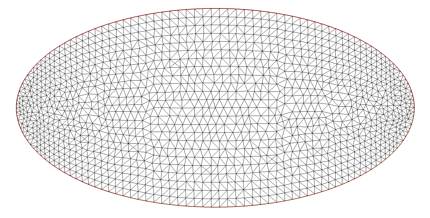
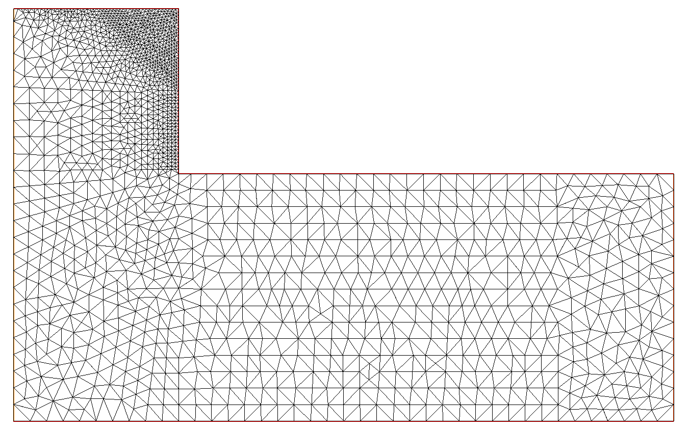
real aL=8., bL=3., cL=2, dL=2., aE = 0.49*aL, bE = 0.49*bL; // geometry
// Define region border
border B1(t=0,aL) { x = t; y=0; label=1; }
border B2(t=0,bL) { x = aL; y=t; label=2; }
border B3(t=0,aL-cL) { x = aL-t; y=bL; label=1; }
border B4(t=0,dL) { x = cL; y=bL+t; label=1; }
border B5(t=0,cL) { x = cL-t; y=bL+dL; label=1; }
border B6(t=0,bL+dL) { x = 0; y=bL+dL-t; label=3; }

int n=5; // Choose base boundary discretization 
// Generate mesh of region interior mesh Th=buildmesh(B1(8*n)+B2(3*n)+B3(6*n)+B4(10*n)+B5(10*n)+B6(5*n));
plot(Th,wait=true, ps="Lshape.eps");

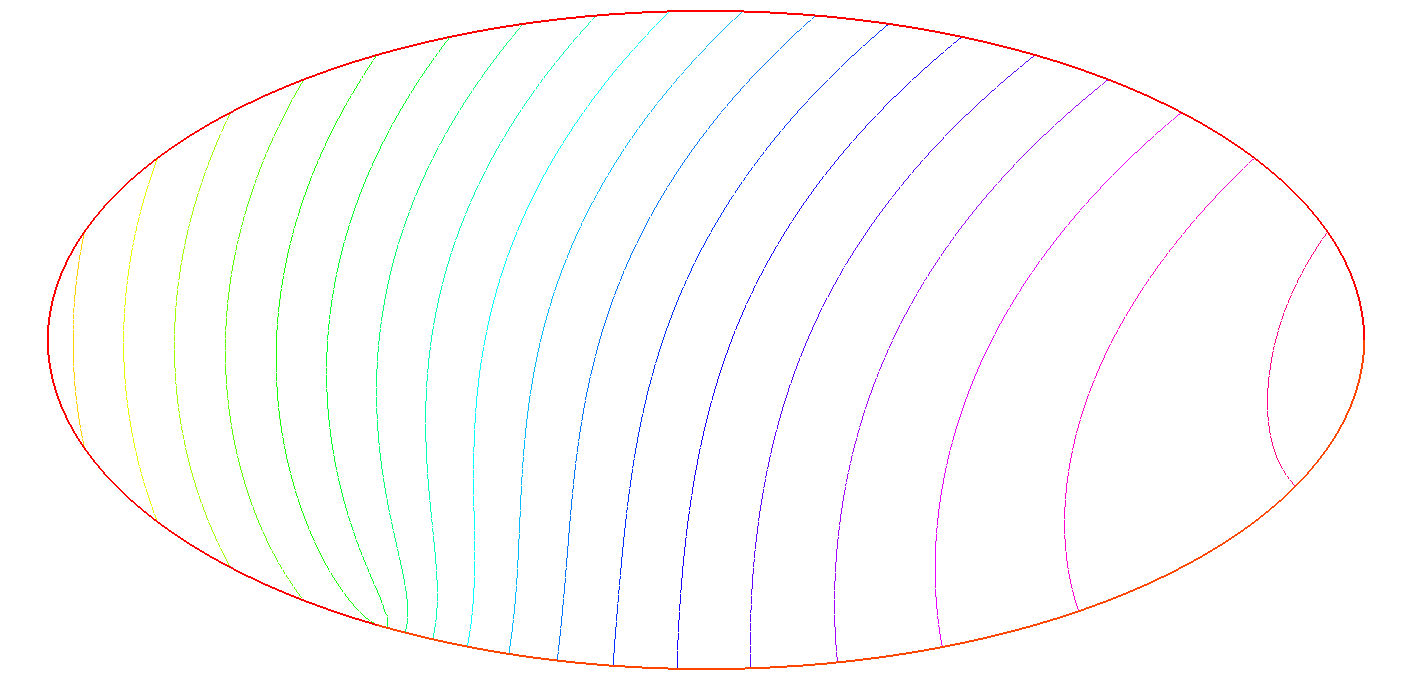
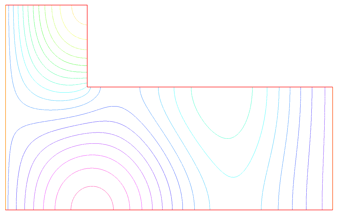
real k2=1.; // Wavenumber 
Vh(Th,P2); // Define finite element space, test functions fespace 
Vh u,v;
// Weak form of Helmholtz operator solve
Helmholtz(u,v) = int2d(Th)(dx(u)*dx(v) + dy(u)*dy(v) - k2*u*v) +
                 on(2,u=1) + on(3,u=0) ;

plot(u, wait=true, ps="Lmode.eps"); // Display eigenmode 

Helmholtz problem: generating linear system

// Build Helmholtz problem discretization
varf vHelmholtz(u,v) = int2d(Th)(dx(u)*dx(v) + dy(u)*dy(v) - k2*u*v) +
       on(2,u=2) + on(3,u=0);

matrix A = vHelmholtz(Vh,Vh);
real[int] b = vHelmholtz(0,Vh);

// Save the discretization to a file
{ofstream fout("A.txt"); fout << A << endl;}
{ofstream fout("b.txt"); fout << b << endl;}