MATH761

MATH76109/21/2018

Lab04: Finite difference schemes for hyperbolic equations

1Semi-discretization

Semi-discretization of the advection equation

q_{t} + u q_{x} = 0

using a centered difference scheme leads to the ODE system

\frac{d}{d t} 𝑸 = - \frac{u}{2 h} 𝐁 𝑸

with $𝐁 = diag ([\begin{array}{lll} - 1 & 0 & 1 \end{array}])$ . We consider the solution of the above ODE system by:

Forward Euler (FTCS scheme)
$𝑸^{n + 1} = (𝑰 - \frac{ν}{2} 𝐁) 𝑸^{n}$
with $ν = u k / h$ known as the CFL number.
Midpoint (leap-frog scheme)
$𝑸^{n + 1} = 𝑸^{n - 1} - ν 𝐁 𝑸^{n}$
Lax-Friedrichs
$𝑸^{n + 1} = (𝝁 - \frac{ν}{2} 𝐁) 𝑸^{n}$
with $𝝁 = \frac{1}{2} (diag ([\begin{array}{lll} 1 & 0 & 0 \end{array}]) + diag ([\begin{array}{lll} 0 & 0 & 1 \end{array}]))$ the averaging operator
Lax-Wendroff
$𝑸^{n + 1} = (𝑰 - \frac{ν}{2} 𝐁 + \frac{ν^{2}}{2} 𝐃) 𝑸^{n}$
with $𝐃 = diag ([\begin{array}{lll} 1 & - 2 & 1 \end{array}])$

This Lab introduces a number of useful techniques:

linking efficient compiled implementations (in Fortran) to an interpreted language (Python), and thus develop an environment for interactive investigation of behavior of numerical schemes;
literate programming within TeXmacs;
development of a Makefile to automate common tasks

Literate programming is the simultaneous development of code implementing an algorithm with construction of full documentation of the underlying mathematics. Within this document tabular material such as the following examples contains code in the left column and comments on the code in the right column. The following block can be copy/pasted to generate additional blocks.

Fortran comments start with !

C++ comments start with //

Python comments start with #

The ./lab04/Makefile extracts verbatim all code within the Fortran-code TeXmacs environment into a lab04.f90 file that is compiled into a Python-loadable module by the f2py utility. The TeXmacs file is first converted to LaTeX, after which the awk utility is invoked to extract text within the tmcode[fortran] environment.

./lab04/Makefile:

2Implementation

2.1Global definitions

A module is constructed with global definitions.

SELECTED_REAL_KIND(P,R) is a Fortran intrinsic function that returns the available type closest to the requested precision of P decimal digits and an exponent range R. Two, possibly different, precisions are defined for the dependent variables ( $q$ ) and the independent variables (space, time).

2.2Time stepping

	A common interface to all finite difference schemes: method: scheme to apply m: number of interior nodes nSteps: number of time steps cfl: CFL number Q0,Q1: initial conditions Q: final state after time stepping Qlft: boundary values at left Qrgt: boundary values at right
	Internal variable declarations
	Precomputation of common expresions
	Start of SELECT statement

Carry out time steps.

For $u > 0$ , use specified left boundary value, extrapolate at right. For $u < 0$ use specified right boundary value, extrapolate at left.

$Q_{i}^{n + 1} = Q_{i}^{n} - \frac{ν}{2} (Q_{i + 1}^{n} - Q_{i - 1}^{n})$

$Q_{i}^{n + 1} = Q_{i}^{n} - ν (Q_{i}^{n} - Q_{i - 1}^{n})$ for $u > 0$

$Q_{i}^{n + 1} = Q_{i}^{n} - ν (Q_{i + 1}^{n} - Q_{i}^{n})$ for $u < 0$

$Q_{i}^{n + 1} = Q_{i}^{n - 1} - ν (Q_{i + 1}^{n} - Q_{i - 1}^{n})$

$Q_{i}^{n + 1} = Q_{i}^{n - 1} - \frac{ν}{2} (Q_{i + 1}^{n} - Q_{i - 1}^{n}) + \frac{ν^{2}}{2} (Q_{i + 1}^{n} - 2 Q_{i}^{n} + Q_{i - 1}^{n})$

3Numerical experiments

Compilation of the above implementation leads to a Python-loadable module than can be used for numerical experiments.

Python]

from pylab import *

Python]

import os,sys

os.chdir('/home/student/courses/MATH761/lab04')

cwd=os.getcwd()

sys.path.append(cwd)

Python]

from lab04 import *

Python]

print scheme.__doc__

q = scheme(method,cfl,q0,q1,qlft,qrgt,[m,nsteps])


Wrapper for ‘‘scheme‘‘.

Parameters
----------
method : input int
cfl : input float
q0 : in/output rank-1 array('d') with bounds (m + 2)
q1 : in/output rank-1 array('d') with bounds (m + 2)
qlft : input rank-1 array('d') with bounds (nsteps + 1)
qrgt : input rank-1 array('d') with bounds (nsteps + 1)

Other Parameters
----------------
m : input int, optional
    Default: (len(q0)-2)
nsteps : input int, optional
    Default: (len(qlft)-1)

Returns
-------

q : rank-1 array('d') with bounds (m + 2)

Python]

3.1Smooth boundary condition

The boundary value problem

{\begin{cases} q_{t} + q_{x} = 0, & t > 0, 0 < x < 1 \\ q (t = 0, x) = 0, & 0 ⩽ x ⩽ 1 \\ q (t, x = 0) = g (t) = \sin (2 π κ t), & t > 0 . \end{cases} .

(1)

is a simplified model of the penetration of a wave into a domain from the left.

Python]

def f(x,kappa):

return zeros(size(x))

Python]

def g(t,kappa):

return sin(2*kappa*pi*t)

Python]

m=99; h=1./(m+1); x=arange(m+2)*h;

Python]

u=1;

Python]

FTCS=1; Upwind=2; LaxFriedrichs=3; LeapFrog=4; LaxWendroff=5; BeamWarming=6;

Python]

3.1.1FTCS

The Fortran code can be invoked from within Python for interactive investigation of the behavior of the numerical schemes.

Python]

method=FTCS; nSteps=100; cfl=1; k=h*cfl/u; t=arange(nSteps+1)*k; kappa=4;

Python]

q0=f(x,kappa); q1=zeros(size(x)); Q0=f(x,kappa); Q1=zeros(size(x));

Python]

Qlft=g(t,kappa); Qrgt=zeros(size(t));

Python]

Q1=scheme(method,cfl,Q0,Q1,Qlft,Qrgt);

Python]

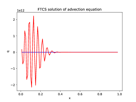
plot(x[1:m],q0[1:m],'b',x[1:m],Q1[1:m],'r');

xlabel('x'); ylabel('q'); title('FTCS solution of advection equation');

savefig("Lab04Fig01.pdf");

Python]

Figure 1. Instability of FTCS scheme

3.1.2Upwind

More importantly, the Fortran code can be included in Python loops to study the influence of discretization parameters. For example, the predictions of a scheme at different CFL numbers can be investigated. Note that all Python commands are now grouped in a single input field to be executed together, thus allowing efficient modification of initial, boundary conditions, numerical parameters.

Python]

method=Upwind;

m=99; h=1./(m+1); x=arange(m+2)*h;

dcfl=0.1; tfinal=0.5;

clf();

qex=g(tfinal-x/u,kappa);

plot(x[1:m],qex[1:m],'k.');

for cfl in arange(dcfl,1+dcfl,dcfl):

k=h*cfl/u; nSteps=ceil(tfinal/k); t=arange(nSteps+1)*k; kappa=4;

Q0=f(x,kappa); Q1=zeros(size(x));

Qlft=g(t,kappa); Qrgt=zeros(size(t));

Q1=scheme(method,cfl,Q0,Q1,Qlft,Qrgt);

plot(x[1:m],Q1[1:m],'b');

xlabel('x'); ylabel('q'); title('Effect of CFL upon Upwind solution of advection equation');

savefig("Lab04UpwindSmoothInitCond.pdf");

Python]

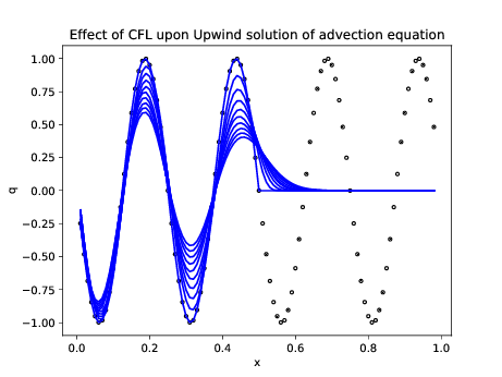Figure 2. Upwind scheme exhibits large artificial diffusion for $CFL < 1$ .

3.1.3Leapfrog

Python]

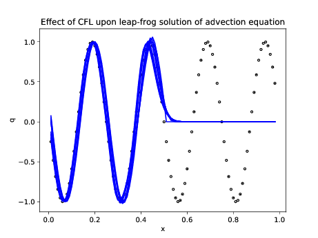
method=LeapFrog;

m=99; h=1./(m+1); x=arange(m+2)*h;

dcfl=0.1; tfinal=0.5;

clf();

qex=g(tfinal-x/u,kappa);

plot(x[1:m],qex[1:m],'k.');

for cfl in arange(dcfl,1+dcfl,dcfl):

k=h*cfl/u; nSteps=ceil(tfinal/k); t=arange(nSteps+1)*k; kappa=4;

Q0=f(x-u*k,kappa); Q1=f(x,kappa);

Qlft=g(t,kappa); Qrgt=zeros(size(t));

Q1=scheme(method,cfl,Q0,Q1,Qlft,Qrgt);

plot(x[1:m],Q1[1:m],'b');

xlabel('x'); ylabel('q'); title('Effect of CFL upon leap-frog solution of advection equation');

savefig("Lab04LeapFrogSmoothInitCond.pdf");

Python]

Figure 3. Upwind scheme

3.1.4Lax-Wendroff

Python]

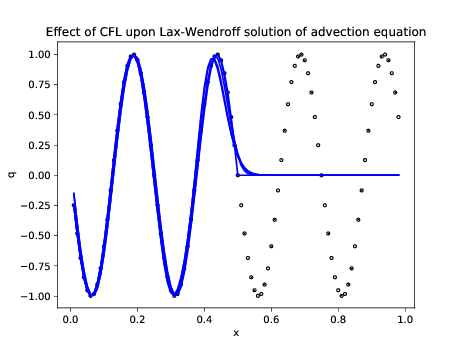
method=LaxWendroff;

m=99; h=1./(m+1); x=arange(m+2)*h;

dcfl=0.2; tfinal=0.5;

clf();

qex=g(tfinal-x/u,kappa);

plot(x[1:m],qex[1:m],'k.');

for cfl in arange(dcfl,1+dcfl,dcfl):

k=h*cfl/u; nSteps=ceil(tfinal/k); t=arange(nSteps+1)*k; kappa=4;

Q0=f(x,kappa); Q1=zeros(size(x));

Qlft=g(t,kappa); Qrgt=zeros(size(t));

Q1=scheme(method,cfl,Q0,Q1,Qlft,Qrgt);

plot(x[1:m],Q1[1:m],'b');

xlabel('x'); ylabel('q'); title('Effect of CFL upon Lax-Wendroff solution of advection equation');

savefig("Lab04LaxWendroffSmoothInitCond.pdf");

Python]

Figure 4. Lax-Wendroff

3.2Discontinuous boundary condition

Study now the behavior for a discontinuous (shock) initial condition

Python]

def f(x,kappa):

return zeros(size(x))

def g(t,kappa):

return (sign(t)+1)/2

u=1;

Python]

kappa=4

Python]

3.2.1Upwind

Python]

method=Upwind;

m=99; h=1./(m+1); x=arange(m+2)*h;

dcfl=0.1; tfinal=0.5;

clf();

qex=g(tfinal-x/u,kappa);

plot(x[1:m],qex[1:m],'k.');

for cfl in arange(dcfl,1+dcfl,dcfl):

k=h*cfl/u; nSteps=ceil(tfinal/k); t=arange(nSteps+1)*k; kappa=4;

Q0=f(x,kappa); Q1=zeros(size(x));

Qlft=g(t,kappa); Qrgt=zeros(size(t));

Q1=scheme(method,cfl,Q0,Q1,Qlft,Qrgt);

plot(x[1:m],Q1[1:m],'b');

xlabel('x'); ylabel('q'); title('Shock propagation by upwind scheme');

savefig("Lab04UpwindShockInitCond.pdf");

Python]

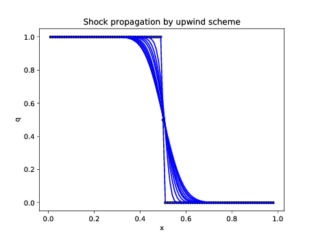Figure 5. Upwind scheme exhibits diffusion but predicts correct shock position

3.2.2Leapfrog

Python]

method=LeapFrog;

m=99; h=1./(m+1); x=arange(m+2)*h;

dcfl=0.2; tfinal=0.5;

clf();

qex=g(tfinal-x/u,kappa);

plot(x[1:m],qex[1:m],'k.');

for cfl in arange(dcfl,1+dcfl,dcfl):

k=h*cfl/u; nSteps=ceil(tfinal/k); t=arange(nSteps+1)*k; kappa=4;

Q0=f(x-u*k,kappa); Q1=f(x,kappa);

Qlft=g(t,kappa); Qrgt=zeros(size(t));

Q1=scheme(method,cfl,Q0,Q1,Qlft,Qrgt);

plot(x[1:m],Q1[1:m],'b');

xlabel('x'); ylabel('q'); title('Shock propagation by leap-frog scheme');

savefig("Lab04LeapFrogShockInitCond.pdf");

Python]

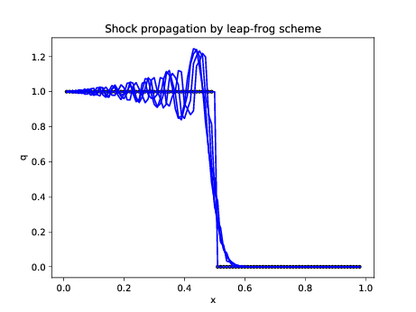Figure 6. Leap-frog exhibits artificial diffusion, dispersion, Gibbs oscillations

3.2.3Lax-Wendroff

Python]

method=LaxWendroff;

m=99; h=1./(m+1); x=arange(m+2)*h;

dcfl=0.2; tfinal=0.5;

clf();

qex=g(tfinal-x/u,kappa);

plot(x[1:m],qex[1:m],'k.');

for cfl in arange(dcfl,1+dcfl,dcfl):

k=h*cfl/u; nSteps=ceil(tfinal/k); t=arange(nSteps+1)*k; kappa=4;

Q0=f(x,kappa); Q1=zeros(size(x));

Qlft=g(t,kappa); Qrgt=zeros(size(t));

Q1=scheme(method,cfl,Q0,Q1,Qlft,Qrgt);

plot(x[1:m],Q1[1:m],'b');

xlabel('x'); ylabel('q'); title('Shock propagation by Lax-Wendroff');

savefig("Lab04LaxWendroffShockInitCond.pdf");

Python]

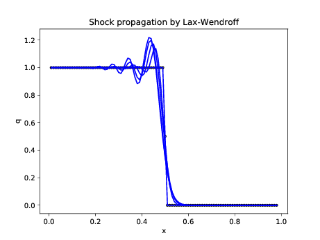Figure 7. Lax-Wendroff is similar to leap-frog with more rapidly decaying Gibbs oscillations