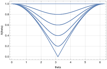
Figure 1. Upwind amplification factor obtained
from Von Neumann analysis
MATH76109/28/2018
Semi-discretization of the advection equation
using a centered difference scheme leads to the ODE system
with . We consider the solution of the above ODE system by:
Forward Euler (FTCS scheme)
with known as the CFL number.
Midpoint (leap-frog scheme)
Lax-Friedrichs
with the averaging operator
Lax-Wendroff
with
Lab05 continues Lab04 by studying the modified equations associated with each of these schemes. The literate programming implementation of Lab04 is expanded to include analysis techniques.
A module is constructed with global definitions.
|
|
|
A common interface to all finite difference schemes: method: scheme to apply m: number of interior nodes nSteps: number of time steps cfl: CFL number Q0,Q1: initial conditions Q: final state after time stepping Qlft: boundary values at left Qrgt: boundary values at right |
|
Internal variable declarations |
|
Precomputation of common expresions |
|
Start of SELECT statement |
|
Carry out time steps. For , use specified left boundary value, extrapolate at right. For use specified right boundary value, extrapolate at left.
|
In[45]:=
Q[n_,j_,theta_] = G[n] Exp[I j theta]
In[46]:=
FTCS = Q[n+1,j,theta] - (Q[n,j,theta] - nu/2
(Q[n,j+1,theta]-Q[n,j-1,theta]))
In[47]:=
expr = Expand[FTCS/G[n]] /. G[n+1]/G[n]->A
In[48]:=
AmpFact[theta_] = Simplify[ComplexExpand[A /. Solve[expr
== 0,A][[1,1]]]]
In[49]:=
The amplifcation factor is , hence the FTCS method is always unstable.
In[10]:=
FTCS = s[t+k,x] - (s[t,x] - nu/2 (s[t,x+h]-s[t,x-h]))
In[14]:=
mFTCS = Simplify[Normal[Series[FTCS,{k,0,2},{h,0,2}]]]
From above series expansions find the modified equation
an advection-diffusion equation with negative diffusivity, again indicating instability of the FTCS method.
|
for
for |
In[87]:=
Upwind = Q[n+1,j,theta] - (Q[n,j,theta] - nu
(Q[n,j,theta]-Q[n,j-1,theta]))
In[88]:=
expr = Expand[Upwind/G[n]] /. G[n+1]/G[n]->A
In[89]:=
AmpFact[theta_] = Simplify[TrigReduce[ComplexExpand[A /.
Solve[expr == 0,A][[1,1]]]]]
In[90]:=
A[theta_,nu_]=Sqrt[TrigReduce[ComplexExpand[AmpFact[theta]
Conjugate[AmpFact[theta]]]]]
In[93]:=
UpwindStabPlot=Plot[Table[A[theta,nu],{nu,0.1,1.0,0.1}],{theta,0,2Pi},
GridLines->Automatic,Axes->False,Frame->True,FrameLabel->{"theta","A(theta)"}];
Export["/home/student/courses/MATH761/lab05/UpwindStabPlot.pdf",UpwindStabPlot]
In[94]:=
|
Figure 1. Upwind amplification factor obtained
from Von Neumann analysis
|
In[94]:=
Upwind = s[t+k,x] - (s[t,x] - nu (s[t,x]-s[t,x-h]))
In[96]:=
mUpwind = Simplify[Normal[Series[Upwind,{k,0,2},{h,0,2}]]]
In[97]:=
From above series expansions find the modified equation
again an advection-diffusion equation with diffusivity
Note that the diffusivity is zero at CFL . The analytical solution to
is
In[99]:=
s[t_,x_]=(1+Erf[(x-u t)/Sqrt[4 alpha t]])/2
In[100]:=
Simplify[ D[s[t,x],t] + u D[s[t,x],x] - alpha
D[s[t,x],{x,2}] ]
In[101]:=
|
|
|
|
|
|
Compilation of the above implementation leads to a Python-loadable module than can be used for numerical experiments.
from pylab import *
Python]
import os,sys
os.chdir('/home/student/courses/MATH761/lab05')
cwd=os.getcwd()
sys.path.append(cwd)
Python]
from lab05 import *
Python]
print scheme.__doc__
Python]
q = scheme(method,cfl,q0,q1,qlft,qrgt,[m,nsteps])
Wrapper for ‘‘scheme‘‘.

Parameters
----------
method : input int
cfl : input float
q0 : in/output rank-1 array('d') with bounds (m + 2)
q1 : in/output rank-1 array('d') with bounds (m + 2)
qlft : input rank-1 array('d') with bounds (nsteps + 1)
qrgt : input rank-1 array('d') with bounds (nsteps + 1)

Other Parameters
----------------
m : input int, optional
    Default: (len(q0)-2)
nsteps : input int, optional
    Default: (len(qlft)-1)

Returns
-------
q : rank-1 array('d') with bounds (m + 2)
Python]
Study now the behavior for a discontinuous (shock) initial condition . The upwind solution will be compared to the exact solution for the advection equation , and the exact solution
to the modified equation , with artificial diffusivity
def f(x,kappa):
return zeros(size(x))
def g(t,kappa):
return (sign(t)+1)/2
u=1;
Python]
FTCS=1; Upwind=2; LaxFriedrichs=3; LeapFrog=4;
LaxWendroff=5; BeamWarming=6;
Python]
kappa=4
Python]
Python]
method=Upwind
from math import erf
m=99; h=1./(m+1); x=arange(m+2)*h;
dcfl=0.2; tfinal=0.5;
clf();
qex=g(tfinal-x/u,kappa);
plot(x[1:m],qex[1:m],'k.'); s = zeros(size(x));
for cfl in arange(dcfl,1+dcfl,dcfl):
k=h*cfl/u; nSteps=ceil(tfinal/k); t=arange(nSteps+1)*k;
kappa=4;
Q0=f(x,kappa); Q1=zeros(size(x));
Qlft=g(t,kappa); Qrgt=zeros(size(t));
Q1=scheme(method,cfl,Q0,Q1,Qlft,Qrgt);
alpha = max(cfl*h**2*(1-cfl)/(2*k),10**(-6));
y = (u*tfinal-x)/sqrt(4*alpha*tfinal);
for i in range(m+1):
s[i] = 0.5*(1+erf(y[i]));
plot(x[1:m],Q1[1:m],'b',x[1:m],s[1:m],'r.');
xlabel('x'); ylabel('q'); title('Shock propagation by
upwind scheme');
savefig("Lab05UpwindShockInitCond.pdf");
Python]
Python]
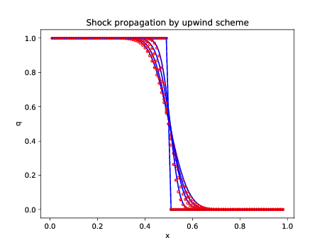 |
Figure 2. The exact solution to the modified
equation corresponds closely to the results from the upwind scheme
|