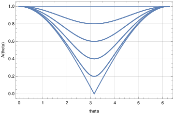
Figure 1. Upwind amplification factor obtained
from Von Neumann analysis
MATH76110/05/2018
Semi-discretization of the consdervation equation
leads to the linearized ODE system
that can be integrated in time using standard schemes. The methods are similar to those obtained in the one spatial dimension case. As an example, we'll consider the midpoint (leap-frog scheme)
Taylor series expansion to second-order accuracy:
The linearized equation leads to the solution
The formal solution can be approximated by
or to higher order (Strang-splitting)
A module is constructed with global definitions.
|
|
|
A common interface to all finite difference schemes: method: scheme to apply m: number of interior nodes nSteps: number of time steps cfl: CFL number Q0,Q1: initial conditions Q: final state after time stepping Qlft: boundary values at left Qrgt: boundary values at right |
|
Internal variable declarations |
|
Precomputation of common expresions |
|
Start of SELECT statement |
|
Carry out time steps. For , use specified left boundary value, extrapolate at right. For use specified right boundary value, extrapolate at left.
|
In[45]:=
Q[n_,j_,theta_] = G[n] Exp[I j theta]
In[46]:=
FTCS = Q[n+1,j,theta] - (Q[n,j,theta] - nu/2
(Q[n,j+1,theta]-Q[n,j-1,theta]))
In[47]:=
expr = Expand[FTCS/G[n]] /. G[n+1]/G[n]->A
In[48]:=
AmpFact[theta_] = Simplify[ComplexExpand[A /. Solve[expr
== 0,A][[1,1]]]]
In[49]:=
The amplifcation factor is , hence the FTCS method is always unstable.
In[10]:=
FTCS = s[t+k,x] - (s[t,x] - nu/2 (s[t,x+h]-s[t,x-h]))
In[14]:=
mFTCS = Simplify[Normal[Series[FTCS,{k,0,2},{h,0,2}]]]
From above series expansions find the modified equation
an advection-diffusion equation with negative diffusivity, again indicating instability of the FTCS method.
|
for
for |
In[87]:=
Upwind = Q[n+1,j,theta] - (Q[n,j,theta] - nu
(Q[n,j,theta]-Q[n,j-1,theta]))
In[88]:=
expr = Expand[Upwind/G[n]] /. G[n+1]/G[n]->A
In[89]:=
AmpFact[theta_] = Simplify[TrigReduce[ComplexExpand[A /.
Solve[expr == 0,A][[1,1]]]]]
In[90]:=
A[theta_,nu_]=Sqrt[TrigReduce[ComplexExpand[AmpFact[theta]
Conjugate[AmpFact[theta]]]]]
In[93]:=
UpwindStabPlot=Plot[Table[A[theta,nu],{nu,0.1,1.0,0.1}],{theta,0,2Pi},
GridLines->Automatic,Axes->False,Frame->True,FrameLabel->{"theta","A(theta)"}];
Export["/home/student/courses/MATH761/lab05/UpwindStabPlot.pdf",UpwindStabPlot]
In[94]:=
|
Figure 1. Upwind amplification factor obtained
from Von Neumann analysis
|
In[94]:=
Upwind = s[t+k,x] - (s[t,x] - nu (s[t,x]-s[t,x-h]))
In[96]:=
mUpwind = Simplify[Normal[Series[Upwind,{k,0,2},{h,0,2}]]]
In[97]:=
From above series expansions find the modified equation
again an advection-diffusion equation with diffusivity
Note that the diffusivity is zero at CFL . The analytical solution to
is
In[99]:=
s[t_,x_]=(1+Erf[(x-u t)/Sqrt[4 alpha t]])/2
In[100]:=
Simplify[ D[s[t,x],t] + u D[s[t,x],x] - alpha
D[s[t,x],{x,2}] ]
In[101]:=
|
|
|
|
|
|
Compilation of the above implementation leads to a Python-loadable module than can be used for numerical experiments.
from pylab import *
Python]
import os,sys
os.chdir('/home/student/courses/MATH761/lab05')
cwd=os.getcwd()
sys.path.append(cwd)
Python]
from lab05 import *
Python]
print scheme.__doc__
Python]
q = scheme(method,cfl,q0,q1,qlft,qrgt,[m,nsteps])
Wrapper for ‘‘scheme‘‘.

Parameters
----------
method : input int
cfl : input float
q0 : in/output rank-1 array('d') with bounds (m + 2)
q1 : in/output rank-1 array('d') with bounds (m + 2)
qlft : input rank-1 array('d') with bounds (nsteps + 1)
qrgt : input rank-1 array('d') with bounds (nsteps + 1)

Other Parameters
----------------
m : input int, optional
    Default: (len(q0)-2)
nsteps : input int, optional
    Default: (len(qlft)-1)

Returns
-------
q : rank-1 array('d') with bounds (m + 2)
Python]
Study now the behavior for a discontinuous (shock) initial condition . The upwind solution will be compared to the exact solution for the advection equation , and the exact solution
to the modified equation , with artificial diffusivity
def f(x,kappa):
return zeros(size(x))
def g(t,kappa):
return (sign(t)+1)/2
u=1;
Python]
FTCS=1; Upwind=2; LaxFriedrichs=3; LeapFrog=4;
LaxWendroff=5; BeamWarming=6;
Python]
kappa=4
Python]
Python]
method=Upwind
from math import erf
m=99; h=1./(m+1); x=arange(m+2)*h;
dcfl=0.2; tfinal=0.5;
clf();
qex=g(tfinal-x/u,kappa);
plot(x[1:m],qex[1:m],'k.'); s = zeros(size(x));
for cfl in arange(dcfl,1+dcfl,dcfl):
k=h*cfl/u; nSteps=ceil(tfinal/k); t=arange(nSteps+1)*k;
kappa=4;
Q0=f(x,kappa); Q1=zeros(size(x));
Qlft=g(t,kappa); Qrgt=zeros(size(t));
Q1=scheme(method,cfl,Q0,Q1,Qlft,Qrgt);
alpha = max(cfl*h**2*(1-cfl)/(2*k),10**(-6));
y = (u*tfinal-x)/sqrt(4*alpha*tfinal);
for i in range(m+1):
s[i] = 0.5*(1+erf(y[i]));
plot(x[1:m],Q1[1:m],'b',x[1:m],s[1:m],'r.');
xlabel('x'); ylabel('q'); title('Shock propagation by
upwind scheme');
savefig("Lab05UpwindShockInitCond.pdf");
Python]
Python]
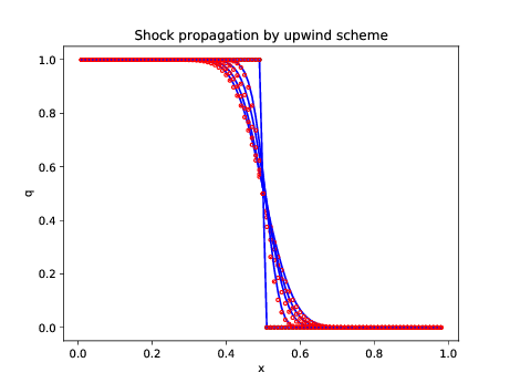 |
Figure 2. The exact solution to the modified
equation corresponds closely to the results from the upwind scheme
|